
Mahony AHRS and Online Gyroscope Bias Estimation
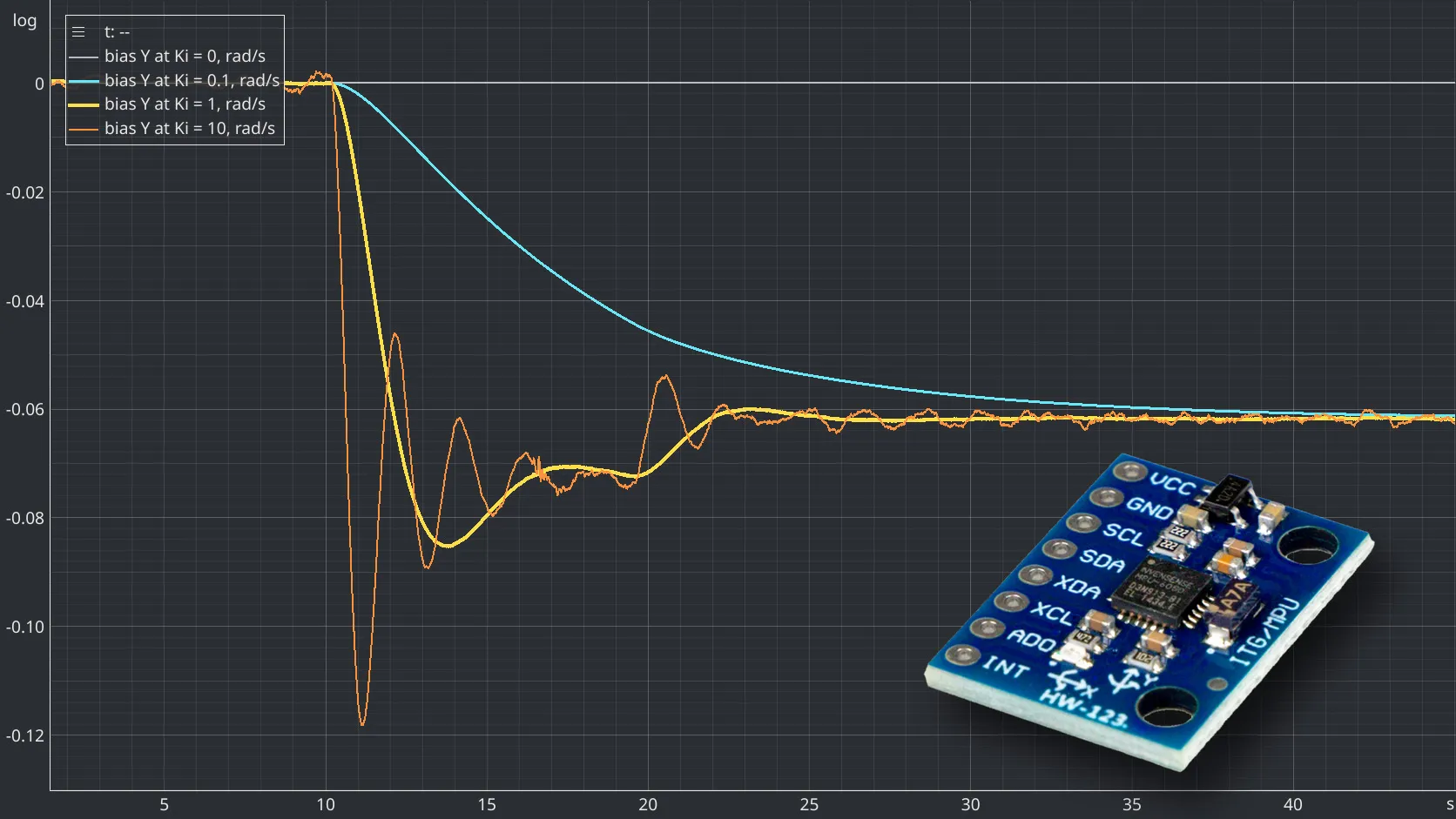
Adding integral feedback to the quaternion estimator from experiment 010 so that it learns a gyroscope bias while the firmware keeps running. Four integral gains ran side by side on the same samples while a known offset was written into the gyroscope calibration by hand. The estimates reached 88 and 81 percent of the offset on two axes and had the opposite sign on the third, and the shortfall matched the one component of the bias that gravity cannot show.
Published
A gyroscope bias that changes after startup cannot always be corrected with a calibration value measured beforehand. This experiment adds integral feedback to the quaternion attitude estimator from Experiment #010 and investigates whether the estimator can learn that changing bias while the sensor is running.
The interesting part is not simply that the additional term reduces drift. It is understanding what the integral term actually estimates, how its behaviour compares with a conventional PI controller, and why even a converged estimate cannot necessarily correct all three gyroscope axes.
1. The Problem: A Good Calibration Does Not Stay Perfect
The previous experiments established two important facts about the MPU6050.
First, the gyroscope reports angular velocity with an offset even when the sensor is stationary. Integrating this offset produces an orientation error that grows with time.
Second, a quaternion-based attitude estimator can use the accelerometer’s measurement of gravity to correct orientation errors. The proportional feedback introduced in Experiment #010 continuously compares the estimated gravity direction with the measured direction and applies an angular-velocity correction.
That correction is effective, but it has a limitation. A proportional controller needs a persistent error to produce a persistent correction. If a gyroscope bias remains, the estimator may settle with a non-zero gravity-direction error.
What happens if the sensor’s bias changes after calibration? Can the estimator adapt without stopping the firmware, measuring the bias again, or restarting the device?
This experiment adds an integral term to investigate that question.
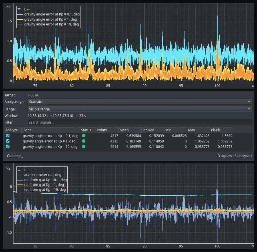 Figure 1 — The limitation, measured in experiment #010. Once the loop has settled, the angle between the measured and the estimated gravity still averages 0.640° at Kp = 0.1 and 0.182° at Kp = 1. A proportional loop leaves a standing error, and the weaker the gain, the larger it is.
2. From Proportional Feedback to a PI Controller
Experiment #010 introduced a feedback loop around the quaternion attitude estimate. The gyroscope propagates the orientation, while the accelerometer supplies a reference direction through gravity.
Let be the normalized accelerometer measurement and the gravity direction predicted by the current quaternion. Their cross product provides an error vector:
The sign of this error depends on the chosen coordinate and cross-product conventions. The correction equations must use a consistent convention throughout the implementation.
The proportional correction is:
It converts the direction error into an angular-velocity correction. A larger produces a stronger response to the same error.
However, proportional feedback does not remember past errors. If a constant disturbance requires a constant correction, a proportional-only loop generally needs a non-zero error to maintain that correction.
What the integral term adds
A conventional PI controller combines proportional and integral actions:
The proportional term responds to the error now. The integral term accumulates error over time, allowing the controller to develop a sustained correction even when the instantaneous error becomes small.
Mahony’s attitude observer uses the same basic feedback idea. In this application, however, the integral term has a particularly useful interpretation: it estimates a slowly varying gyroscope bias.
A simplified continuous-time representation is:
Here, is the estimated gyroscope bias. The signs shown correspond to the error convention used in this implementation. Reversing the error-vector convention requires corresponding changes to the correction signs.
The bias estimate is updated incrementally:
The corrected angular velocity is then used in the same quaternion integration process as before.
The important point is that the integral term does not directly integrate the gyroscope’s measured angular velocity. It integrates the feedback error and uses that accumulated error to estimate a correction to the gyroscope.
How this compares with a PI regulator
The relationship is easiest to understand by separating the mathematical structure from its physical interpretation. Table 1 sets the two side by side.
| Conventional PI regulator | Mahony attitude observer |
|---|---|
| Proportional term reacts to the current control error | corrects the estimated angular velocity |
| Integral term accumulates persistent error | accumulates gravity-direction error |
| Integral output supplies the sustained part of the control action | The integral state acts as an estimate of gyroscope bias |
| The controlled plant determines which errors are observable | The available sensor references determine which bias components are observable |
Table 1 — The two loops side by side, and what each term of a conventional PI regulator corresponds to in the attitude observer.
The two terms are not independent filters, and is not simply a stronger version of . They have different roles and different effects on convergence.
In this implementation, the proportional term supplies an immediate correction, while the integral state changes more gradually. Once the bias estimate has converged, the estimator can compensate for a persistent gyroscope offset without requiring the same persistent gravity-direction error.
There is also an important difference from a generic PI regulator: the integral term cannot estimate what the reference measurements cannot reveal. With only an accelerometer providing the gravity reference, this observer has no absolute heading reference.
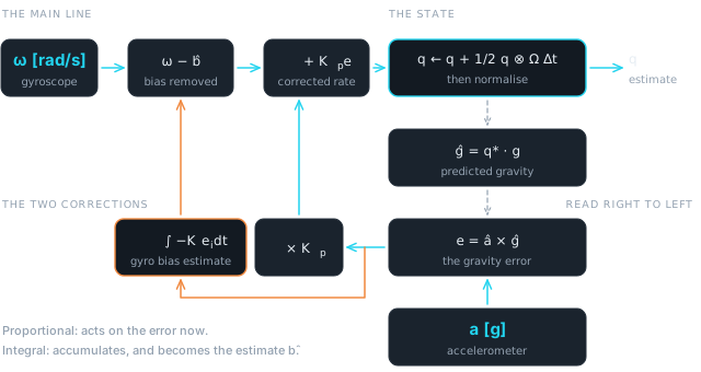 Figure 2 — The same loop as Figure 5 of Experiment #010, with one path added. The gravity error feeds two things: the proportional term, which acts on it at once, and an integrator whose output is the estimated gyroscope bias. This is a schematic, not a capture.
3. Implementation
The existing quaternion propagation remains unchanged. The modification is limited to the feedback path and the additional bias state.
For each update , the estimator performs the following steps. The symbols are those of section 2, with the orientation quaternion, the accelerometer reading, the gravity direction in the world frame and the time since the previous update.
-
Normalize the accelerometer measurement:
-
Calculate the gravity direction predicted by the current quaternion, by rotating the world gravity into the sensor frame with the conjugate:
-
Calculate the gravity-direction error vector:
-
Update the estimated gyroscope bias using the integral term:
-
Subtract the estimated bias from the measured angular velocity. The bias used here is the one just updated in step 4:
-
Apply the proportional correction:
-
Integrate the corrected angular velocity into the quaternion and renormalize:
Steps 4 to 6 together are the discrete form of the two continuous equations in section 2. Written as one line:
The discrete-time bias update is sensitive to the update interval. The factor is essential: changing the execution rate without accounting for it changes the effective integral action.
The proportional and integral gains should also not be interpreted as interchangeable tuning parameters. Increasing strengthens the immediate response to orientation error. Increasing makes the bias estimate adapt more aggressively, which may shorten convergence time but can also increase overshoot and oscillation.
For the implementation tested here, the proportional gain was kept at , and four integral-gain settings were compared:
- : no integral adaptation; used as the baseline.
- : slow, conservative adaptation.
- : intermediate adaptation.
- : aggressive adaptation.
The zero-gain instance is important. It provides a simultaneous comparison with the proportional-only estimator under the same input measurements.
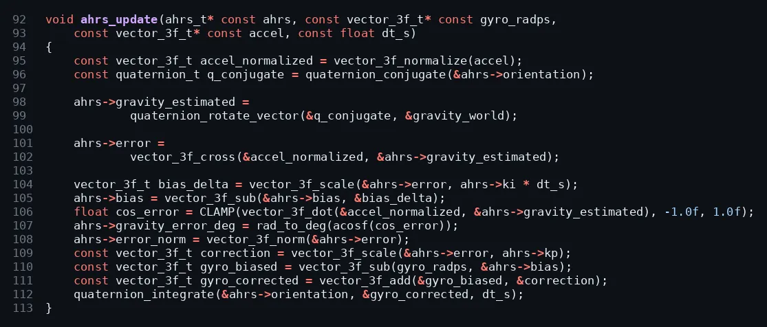 Figure 3 —
ahrs_update() from ahrs.c (lines 92–113), the function every instance runs once per sample. The bias update subtracts ki * dt_s times the error, so the estimate carries the same sign as the offset it cancels, and it is subtracted from the gyroscope before the proportional term is added.
4. Experimental Setup
The experiments use the same hardware platform as the previous articles: an STM32F4 Discovery board and a GY-521 module carrying the MPU6050. The wiring and the sensor configuration are described in detail in Experiment #001.
The firmware reads the sensor and runs the attitude estimators on the microcontroller. EmbedStudio observes the internal variables over SWD while the firmware continues executing.
Two experiments were performed.
The first examines a real thermal disturbance. The sensor was heated, then left stationary while it cooled. The four integral-gain settings were compared during the same recording.
The second applies controlled changes to the gyroscope calibration values while the firmware is running. The values were changed manually through EmbedStudio’s Table instrument over SWD. This produces a known software-side change in the calibration, allowing the estimator’s response to be measured without rebuilding the firmware for every test.
The second experiment is particularly useful because it separates the behaviour of the integral feedback from the slower and less controlled process of sensor heating and cooling.
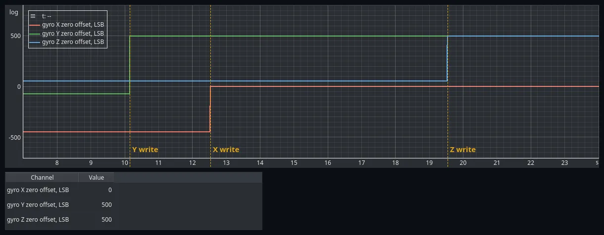 Figure 4 — The three gyroscope zero offsets,
mpu_cal.gyro_bias, written live over SWD from EmbedStudio’s Table instrument. Y was set to 500 LSB at 10.15 s, X to 0 at 12.53 s and Z to 500 LSB at 19.53 s. The Table shows the values after the third write. The firmware did not generate these steps.
5. Experiment A: Thermal Stabilisation
The first experiment introduces a real disturbance rather than a synthetic calibration step. The board was heated for about 25 seconds and then left to cool. It was not touched during the recording, but it was not rigidly mounted either: only the wiring was clamped. It lay tilted, with the accelerometer reading roll and pitch , so gravity had a component along all three sensor axes.
The recording covers 606 seconds, with samples captured at about 97 samples per second. It starts with the estimators already running. The sensor temperature was before heating, started to rise at about 60 s, peaked at at 86.5 s and was back at over the last 20 seconds.
Temperature here is the MPU6050’s reported internal temperature, not an independent measurement of ambient temperature.
The four estimator instances ran in parallel with the same sensor measurements. Their integral gains were , , , and . This makes it possible to compare the estimators without relying on separate runs having identical initial conditions or disturbances.
The gyroscope offset followed the temperature. Between 82 and 92 s, compared with the first 50 s, the calibrated gyroscope read , and on X, Y and Z. That is about 54, 47 and 19 LSB.
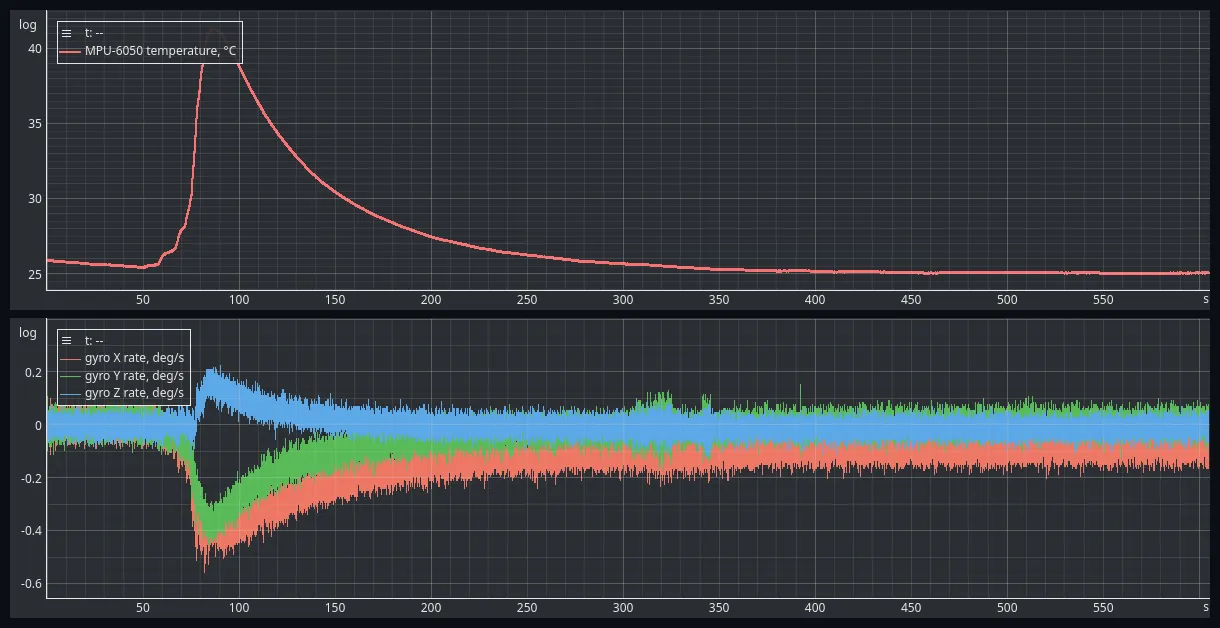 Figure 5 — The thermal recording. Above, the MPU6050’s reported temperature: 25.7 °C, a peak of 41.3 °C at 86.5 s and 25.1 °C at the end. Below, the three calibrated gyroscope rates, with nothing subtracted but the startup calibration. The offset shifts by up to about 0.4 °/s, and X is still at −0.08 °/s at the end, against +0.006 °/s before the heating.
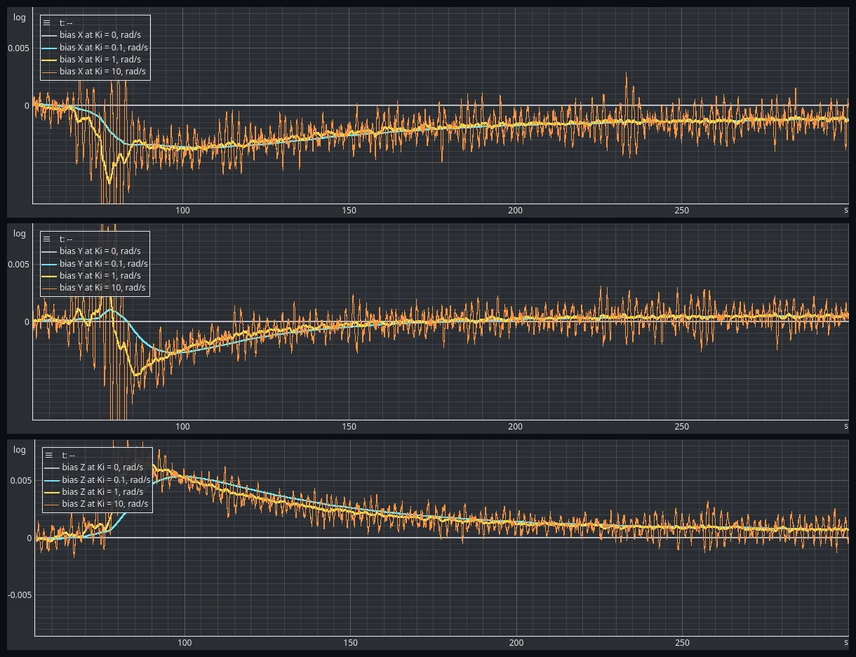 Figure 6 — The bias estimates of the four estimators, one axis per panel, on the same scale. Ki = 0 stays at zero. The other three follow the same curves: down on X and Y and up on Z while the die heats, then back toward zero as it cools. Ki = 0.1 is the smoothest and the latest. Ki = 10 is the noisy trace, and it goes off scale during the heating.
The question is whether the integral term tracks a changing disturbance, and how closely. The estimator can only see the part of the offset that gravity makes visible, so each estimate is compared with the observable component, calculated as in section 6 from the mean gyroscope reading and the mean accelerometer direction in the same window. Table 2 gives the numbers for three windows.
| Window | Axis | Observable | |||
|---|---|---|---|---|---|
| 82–92 s, 41.0 °C | X | −4.31 | −3.42 | −3.69 | −3.43 |
| Y | −2.91 | −1.21 | −3.76 | −4.00 | |
| Z | +6.05 | +3.79 | +6.33 | +6.29 | |
| 150–160 s, 30.0 °C | X | −2.44 | −2.51 | −2.33 | −2.33 |
| Y | −0.18 | −0.37 | −0.17 | −0.15 | |
| Z | +1.94 | +2.42 | +2.09 | +2.03 | |
| 500–600 s, 25.1 °C | X | −1.09 | −1.01 | −1.01 | −1.02 |
| Y | +0.54 | +0.65 | +0.64 | +0.64 | |
| Z | +0.31 | +0.44 | +0.43 | +0.43 |
Table 2 — Each estimator’s bias, against the observable component of the offset, in three windows of the thermal recording. All values in mrad/s. Observable is the mean gyroscope reading in the window with its component along gravity removed. The other columns are the mean bias estimate of each instance. Ki = 0 reads 0 throughout.
The estimates follow the observable component through the whole drift. Over 200 to 600 s the root-mean-square difference between each estimate and the observable component, taken over 10 s windows, is between 0.09 and 0.16 mrad/s for all three non-zero gains. For the zero-gain instance it is 1.3, 0.5 and 0.5 mrad/s.
The gains differ in how fast they follow and how much noise they carry (Table 3).
| Gravity error at the peak, 82–92 s | RMS error from 60 to 120 s, X / Y / Z | Noise at rest, 500–600 s, X / Y / Z | |
|---|---|---|---|
| 0 | 0.476° | 3.49 / 1.71 / 4.19 | 0 / 0 / 0 |
| 0.1 | 0.242° | 0.68 / 1.15 / 1.46 | 0.02 / 0.02 / 0.02 |
| 1 | 0.092° | 0.62 / 0.91 / 0.39 | 0.11 / 0.10 / 0.08 |
| 10 | 0.098° | 0.88 / 1.00 / 0.25 | 1.04 / 0.89 / 0.66 |
Table 3 — What each integral gain costs and buys in the thermal recording: the gravity error at the peak, how far the estimate was from the observable component while the offset moved, and how much it scattered at rest. The RMS error and the noise are in mrad/s.
The lowest gain was the slowest. At the temperature peak, had reached only 79, 42 and 63 % of the observable offset on X, Y and Z. It took until about 150 s to stay within 0.5 mrad/s of it on all three axes. and took until about 100 s. The gravity error at the peak shows the same gap: 0.476° with no integral action, 0.242° at and about 0.09° at and . Once the board had settled, all three gains ended at about 0.08° and the baseline at 0.10°.
is no better than here, and it is much noisier. At rest its estimate scatters by 0.7 to 1.0 mrad/s, which is 10 to 50 times more than at the lower gains. During the heating it swung as far as 14.7 mrad/s on X and 13.2 on Y, against 3.7 and 2.7 for .
Three things in the recording need a comment. The comparison in Table 2 and the RMS figures above use the whole estimate vector, so they include the third.
- The offset did not return. The die is back below its starting temperature, and X still reads , against before the heating. The MPU6050 is an old and inexpensive part. Its gyroscope offset depends on temperature, but nothing guarantees that it returns to the same value after a thermal cycle. The estimates follow the new offset, which is what a bias estimator is for.
- The tilt changed. The accelerometer’s roll rose from 41.1° to 42.7° at the peak and came back. The board was not mounted rigidly. Only the wiring was clamped, to limit the coupling of vibration, so the board was free to shift as it heated. This is real motion, and an integrator cannot tell motion from bias. It probably adds to the excursions during the heating.
- The settled estimates are slightly off. At rest, each estimate sits 0.08 to 0.13 mrad/s from the observable offset, about 0.006 °/s. Two simple causes can be ruled out. The proportional term is not responsible: with integral action its average contribution is below 0.01 mrad/s, ten times too small. Lag is not responsible either, because all three gains show the same difference. The cause is the direction. The leftover is 0.17 to 0.19 mrad/s long and points along gravity, the one direction the accelerometer cannot see. Perpendicular to gravity, the estimates match the observable offset to within 0.005 mrad/s. The integral term therefore never had a chance to correct it. It probably built up while the board tilted by 1.7° during the heating. The estimate was about 8 mrad/s long then, and 8 mrad/s times 0.03 rad of tilt is about 0.2 mrad/s. This is a plausibility check, not a proof.
6. Experiment B: Applying a Known Gyroscope Offset
The second experiment gives a more controlled way to examine bias estimation.
While the firmware was running, the gyroscope calibration variables were changed manually through EmbedStudio’s Table instrument. The resulting changes in the measured angular-rate signals were checked against the expected changes. The four AHRS instances received the same sensor inputs and used the same proportional gain, while their integral gains differed.
The analysis starts at 5.55 seconds, once the estimators are running. The calibration changes were staggered rather than applied as one simultaneous three-axis step.
The resulting angular-rate offsets were measured as follows (Table 4):
| Axis | Measured rate offset | Equivalent offset |
|---|---|---|
| X | ||
| Y | ||
| Z |
Table 4 — The imposed offset as the gyroscope measured it, in °/s and in rad/s.
The offsets follow from the writes in Figure 4. Y went from −73 to 500 LSB, a change of 573 LSB, and dividing by the Y scale factor of 131.1 LSB per °/s gives 4.371 °/s. X changed by 448 LSB at 132.2, which is 3.389 °/s, and Z by 445 LSB at 130.9, which is 3.399 °/s. The signs are those of the gyroscope’s own reading.
These values describe the imposed software-side disturbance as measured in the gyroscope-rate data. They are the full three-axis offset vector against which the final bias estimate can be compared.
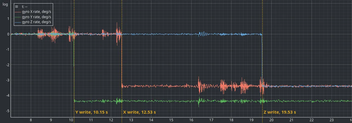 Figure 7 — The calibrated gyroscope rates around the three writes, one axis at a time: Y at 10.15 s, X at 12.53 s and Z at 19.53 s. The dashed lines are painted over the capture at those instants. The bursts of noise on X are small movements of the board, discussed in section 8.
What did the integral term estimate?
At the end of the recording, the three non-zero- instances converged to approximately the following bias estimates (Table 5):
| Axis | Final estimated bias | Full imposed offset |
|---|---|---|
| X | ||
| Y | ||
| Z |
Table 5 — The final bias estimates against the full imposed offset. The Z estimate has the opposite sign.
At first glance, the result looks disappointing. The X and Y estimates do not fully reach the imposed offsets, at 88 % and 81 % of them, and the Z estimate even has the opposite sign.
But the missing part is not necessarily a failure of integral adaptation.
The accelerometer provides a reference for the direction of gravity. That constrains two degrees of orientation freedom: roll and pitch. Rotation about the gravity direction does not change the gravity measurement, so an accelerometer alone cannot provide an absolute heading reference.
As a result, the gyroscope-bias component that produces rotation about gravity is not observable from this reference. The integral estimator can correct the observable component of the offset while an unobservable component remains.
The split can be written down. Let be the unit gravity direction in the sensor frame and the gyroscope bias. The part of the bias that the gravity reference can see is the part perpendicular to , and the rest is the part along it:
This follows from the error vector. Since is perpendicular to , the integral term can only ever change in the plane perpendicular to gravity.
The board was tilted by about 12° from flat. The accelerometer read roll and pitch , which gives . With the imposed offset rad/s, the along-gravity part is rad/s. Removing it leaves the observable component, approximately:
The final estimates from the non-zero- instances matched this derived observable component within approximately .
This is the more meaningful comparison for an accelerometer-only estimator. It does not mean that the full imposed bias was recovered; it means the estimated component agrees with what the gravity reference can constrain under the measured sensor orientation.
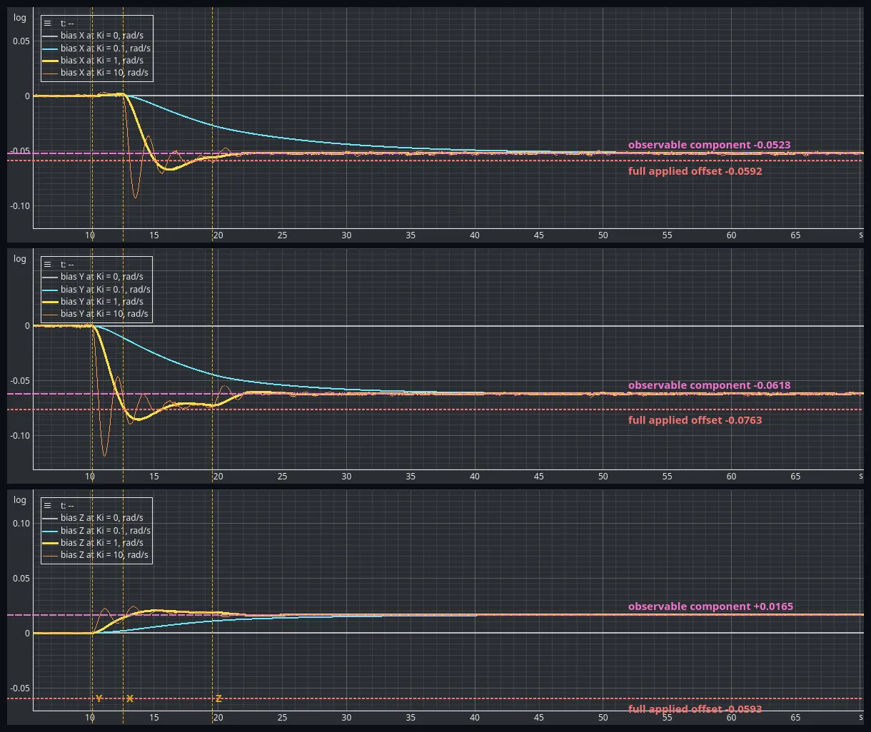 Figure 8 — The three bias components for all four Ki. Dashed pink: the observable component, −0.0523, −0.0618 and +0.0165 rad/s, calculated from the measured gravity direction. Dotted red: the full offset that was applied, −0.0591, −0.0763 and −0.0593 rad/s. Ki = 0.1, 1 and 10 end on the dashed line, not the dotted one. Ki = 0 stays at zero.
What happens to yaw?
The limitation becomes particularly clear in the heading estimate.
For the instance, the final yaw slope was approximately . The slope predicted from the remaining unobservable bias component was approximately .
The prediction is the unobservable part itself. The offset that the integral term cannot see is a rotation rate about gravity, so it is integrated into yaw at that rate:
The close agreement is a useful result. It shows that the residual heading drift is consistent with the part of the bias that the gravity reference cannot determine.
The integral term is not failing to correct an error that it can observe. It is operating with an incomplete reference.
A magnetometer or another independent heading reference is needed to constrain that remaining degree of freedom.
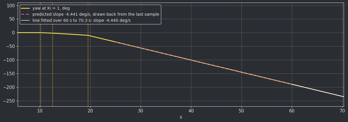 Figure 9 — Yaw of the Ki = 1 estimator, computed from its quaternion; it is the only instance whose quaternion was recorded. From about 25 s the slope is constant. The line fitted over the last 10 s has −4.440 °/s, and the slope predicted from the unobservable component is −4.441 °/s. The yaw reaches −235° by the end. This one is plotted from the capture with a script.
Does the observable part follow the tilt?
The explanation makes a prediction. If the missing part of the bias is the part along gravity, a different tilt must change both what the estimator can see and the yaw drift. So the same test was repeated at two more tilts: the board almost flat, and the board tilted by about 48°. The writes and the gains were the same. The writes changed mpu_cal.gyro_bias by +448 LSB on X, +573 LSB on Y and +444 to +445 LSB on Z, so the imposed offset was the same to within 0.0001 rad/s. For each capture, the prediction was calculated from the gravity direction measured in that capture, not fitted to its estimates.
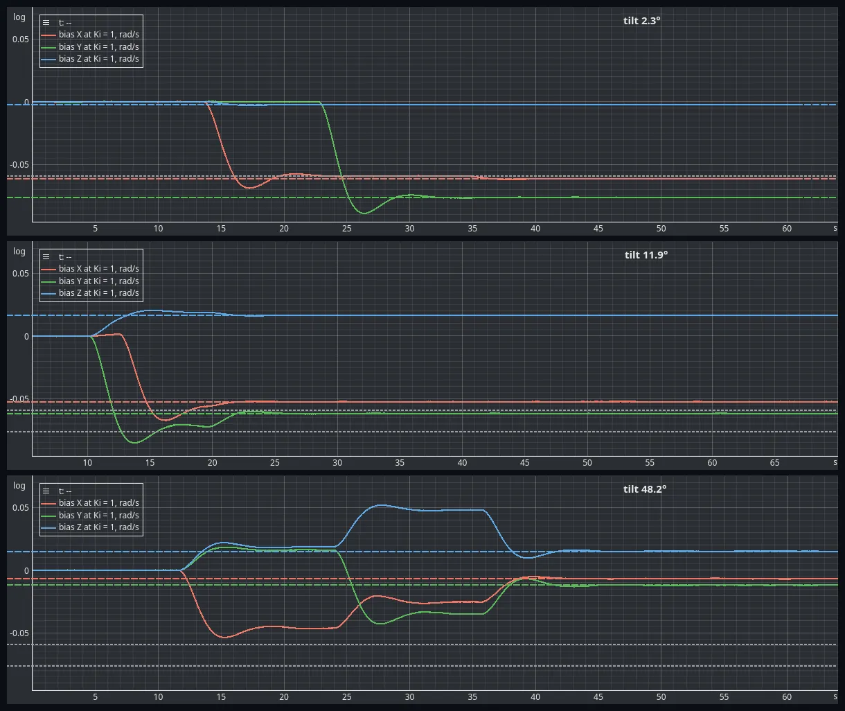 Figure 10 — The X, Y and Z bias estimates of the Ki = 1 instance at three tilts, on the same scale. Dashed, in the axis colours: the observable component calculated for that tilt. Dotted grey: the full X and Y offsets that were applied. At every tilt the estimates settle on the dashed lines. The 11.9° panel is the capture from the start of this section; the other two are new.
| Quantity | 2.3° (almost flat) | 11.9° | 48.2° |
|---|---|---|---|
| Accelerometer roll, pitch | 0.1°, 2.3° | 10.8°, −5.0° | 41.0°, −28.1° |
| Observable part of the offset | 86 % | 73 % | 18 % |
| Observable component X / Y / Z, rad/s | −0.0615 / −0.0763 / −0.0024 | −0.0523 / −0.0618 / +0.0165 | −0.0068 / −0.0118 / +0.0150 |
| Final estimate, , X / Y / Z, rad/s | −0.0614 / −0.0762 / −0.0024 | −0.0524 / −0.0618 / +0.0165 | −0.0067 / −0.0119 / +0.0151 |
| Predicted yaw slope | −3.264 °/s | −4.441 °/s | −6.388 °/s |
| Measured yaw slope, | −3.268 °/s | −4.440 °/s | −6.393 °/s |
Table 6 — The same offset at three tilts. The tilt is the angle of the gravity direction from the sensor’s Z axis. “Observable part” is the length of the observable component divided by the length of the full offset. The predictions use each capture’s own measured gravity direction.
Table 6 gives the numbers. Almost flat, the board sees nearly all of the X and Y offset and almost none of the Z offset. The estimates reach 99.9 % of the observable component on X and Y, and the Z estimate stays at −0.0024 rad/s, not near the −0.0593 rad/s that was applied. The Z offset shows up where the explanation says it should: the yaw drifts at −3.27 °/s, which is the whole Z offset.
At 48° the opposite happens. The board can see only 18 % of the offset. The X and Y estimates end at 11 % and 16 % of the applied offsets, and the Z estimate is positive although the applied Z offset is negative. The yaw drifts at −6.39 °/s.
In all three captures the and estimates match the prediction to within 1 %, and the measured yaw slopes to within 0.005 °/s. A tilt changes the result a lot, and the change is the one calculated from gravity.
These two recordings are shorter than the first one, with 27 to 28 seconds after the last write. and had settled by then. had not: at 48° its X estimate was still at 132 % of its target. The convergence times in Table 7 therefore come from the first capture only.
7. The Cost of Increasing
The integral gain controls how aggressively the estimator adapts its bias estimate (Table 7). The experiment shows that a larger gain does not simply produce a uniformly better result.
| Approximate time to observable target | Observed behaviour | |
|---|---|---|
| 0.1 | 17–24 s | Gradual convergence, no observed overshoot |
| 1 | 8–11 s | Faster convergence, moderate overshoot |
| 10 | 10–11 s | Aggressive response, larger overshoot and oscillation |
Table 7 — Time to settle within ±10 % of the observable component, measured from the first write.
The reported times are approximate and depend on the chosen convergence criterion and the staggered calibration changes. They are measured from the first write, at 10.15 s, to the last time the estimate leaves a band of ±10 % around the observable component. The same criterion applied to the full imposed offset is never met, by any instance, on any axis.
For , convergence was slower but monotonic. For , the estimate reached the target sooner, with some overshoot. For , the response was more oscillatory, with overshoot of approximately to in the analysed components and visible residual wobble.
The high-gain case also illustrates why convergence time alone is not a sufficient tuning criterion. A fast response can come with more overshoot and greater sensitivity to transient disturbances.
The zero-gain baseline, as expected, does not adapt its bias estimate. Its gravity-direction error remains, whereas the non-zero integral-gain instances finish with much smaller changes in roll and pitch relative to their final settled values. The baseline settles 2.7° off in roll and 3.9° off in pitch, which is a standing gravity error of 4.7°. The three others end within 0.02° of where they started.
These results are consistent with the PI interpretation: the integral term develops a sustained correction, but increasing its gain changes the dynamics of the feedback loop. It is not a free improvement.
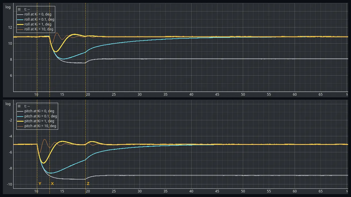 Figure 11 — Roll and pitch of all four instances, on the same axes. Ki = 0 settles 2.7° lower in roll and 3.9° lower in pitch and stays there. Ki = 0.1 comes back slowly and without overshoot, Ki = 1 in roughly ten seconds with one swing, and Ki = 10 fastest, ringing for several cycles.
8. What This Experiment Does—and Does Not—Prove
The results support several conclusions.
- Adding integral feedback allows the estimator to adapt its gyroscope-bias estimate while the firmware continues running.
- The integral gain controls the trade-off between adaptation speed and transient behaviour.
- Repeating the offset test at tilts of 2.3° and 48.2° moved the observable component and the yaw slope as the explanation predicts, to within 1 % and 0.005 °/s.
- On a real thermal drift of up to 0.4 °/s, the estimates followed the observable part of the offset to within about 0.1 mrad/s once the temperature had settled.
- A gravity-only reference constrains the bias component observable through roll and pitch, but it cannot establish absolute heading.
- A remaining yaw drift can therefore be consistent with the unobservable component of the gyroscope bias rather than a failure of the observable bias estimate.
There are also limits to the experiment.
The calibration changes were staggered, so the measurements are not equivalent to one ideal simultaneous step. The host captured snapshots at about 97 Hz while the estimator ran at 1 kHz, so the recorded rows are not atomic snapshots of every internal variable. Brief motion occurred near the calibration changes, and the board was not perfectly level. Each of the three tilts was captured once, without an independent attitude reference. The two extra tilts agreed with the predictions, but there is no repeat at any of them and so no run-to-run spread.
Consequently, the results should not be interpreted as an absolute roll/pitch accuracy measurement or as proof that every bias component will converge under every operating condition.
The observable-component comparison is stronger than comparing the final estimate against the full three-axis offset, but it also depends on the measured gravity direction and the assumptions of the model.
9. Conclusion
Experiment #010 showed how proportional gravity feedback can correct errors in a quaternion attitude estimate. This experiment added integral feedback and showed how the accumulated error can become an online estimate of gyroscope bias.
The connection to a PI controller is useful because it explains the roles of the two gains. The proportional term reacts to the current orientation error; the integral term accumulates that error and supplies a sustained correction through the bias estimate.
The controlled offset experiment also exposed the boundary of what the estimator can know. With only the accelerometer as a reference, the bias component that affects heading cannot be fully determined. A numerically converged bias estimate is therefore not necessarily the complete physical bias vector.
The next step is to investigate an additional attitude-estimation method and, once the magnetometer is available, explore how an independent heading reference changes this limitation.
Source Code and Data
The firmware, analysis scripts, processed data and experimental plots are available in the experiment repository.
The raw captures, the analysis scripts and the processed results are in the EmbedStudio Experiments repository. The firmware is in the release tagged experiment_011.
References
- Experiment #010 — Quaternion Attitude Estimation.
- Mahony, R., Hamel, T., and Pflimlin, J.-M., Nonlinear Complementary Filters on the Special Orthogonal Group, IEEE Transactions on Automatic Control, 2008.
Source Code
The firmware and supporting files for this experiment are available here:
View experiment repository