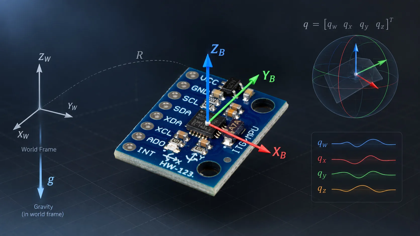
Quaternion Attitude Estimation

Introduction

In the previous experiments, we developed the individual building blocks needed to estimate orientation from an IMU.

In Experiment #008, we integrated the gyroscope measurements to estimate orientation. This demonstrated the fundamental advantage of the gyroscope: it provides a direct measurement of rotational motion. At the same time, the experiment showed the unavoidable problem of integration — even a small gyroscope bias eventually produces significant orientation drift.

In Experiment #009, we combined the gyroscope with the accelerometer using a complementary filter. The gyroscope provided the short-term dynamics, while the accelerometer provided a long-term reference through the direction of gravity.

For that experiment, orientation was represented using Euler angles. This works well for demonstrating the principle, but Euler angles have an inherent weakness: their representation becomes singular around ±90° pitch.

In this experiment, we keep the same basic sensor-fusion idea but change the internal representation of orientation from Euler angles to quaternions.

The goal is not simply to replace one mathematical representation with another. We want to understand why quaternion propagation works, how the accelerometer correction can be applied to it, and whether the resulting estimator behaves better around the problematic ±90° pitch region.

The complete source code and experimental data are available in the public EmbedStudio experiments repository.

Why Move from Euler Angles to Quaternions?

Euler angles describe orientation as three successive rotations:

• roll around the X axis,
• pitch around the Y axis,
• yaw around the Z axis.

This representation is intuitive because the three values correspond directly to angles we can visualize.

The problem is that these three angles are not independent everywhere. Around ±90° pitch, two rotational degrees of freedom become indistinguishable. This is the well-known gimbal-lock singularity.

Importantly, the physical orientation itself does not become singular. Only the Euler-angle representation does.

A quaternion provides an alternative representation that does not have this singularity.

Instead of storing three angles, we represent orientation using four numbers:

$$q = \begin{bmatrix} w & x & y & z \end{bmatrix}$$

For an orientation quaternion, the quaternion is normalized:

$$w^2+x^2+y^2+z^2=1$$

This additional component may initially seem like unnecessary complexity. However, quaternion multiplication provides a particularly convenient way to compose rotations and propagate orientation using angular velocity.

To understand why, we first need to understand what a rotation quaternion actually represents.

Understanding the Quaternion Representation

A unit quaternion representing a rotation by angle $\theta$ around a unit axis $\vec{\mathbf{u}}=(u_x,u_y,u_z)$ is

$$q = \begin{bmatrix} \cos(\theta/2) \\ u_x\sin(\theta/2) \\ u_y\sin(\theta/2) \\ u_z\sin(\theta/2) \end{bmatrix}$$

Or, using the scalar/vector notation,

$$q = \left[ \cos(\theta/2), \vec{\mathbf{u}}\sin(\theta/2) \right]$$

The important detail is the half angle.

For example, a rotation around the X axis is

$$q(\theta)= \begin{bmatrix} \cos(\theta/2)\\ \sin(\theta/2)\\ 0\\ 0 \end{bmatrix}$$

This equation gives us an important intuition: as the physical rotation angle changes, the quaternion moves continuously through its four-dimensional representation.

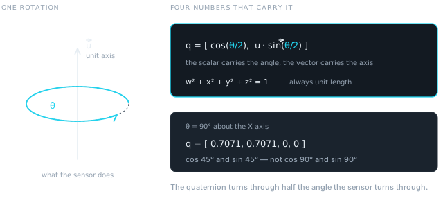Figure 1 — Axis and angle, and the four numbers that carry them. The worked value is not decoration: it is the orientation this experiment’s reset actually writes, and it appears in figure 6.

A useful detailed introduction to this geometric interpretation is provided by J. B. Kuipers in Quaternions and Rotation Sequences. The quaternion visualization material by 3Blue1Brown also provides an intuitive geometric explanation.

How Does the Gyroscope Change a Quaternion?

The gyroscope measures angular velocity:

$$\boldsymbol{\omega} = \begin{bmatrix} \omega_x\\ \omega_y\\ \omega_z \end{bmatrix}$$

The first question is therefore:

How can a three-dimensional angular velocity be used to calculate the change of a four-dimensional quaternion?

We embed the angular velocity vector into a quaternion with zero scalar component:

$$\Omega = \begin{bmatrix} 0\\ \omega_x\\ \omega_y\\ \omega_z \end{bmatrix}$$

This is called a pure quaternion.

It is important not to confuse this quaternion with a rotation quaternion. $\Omega$ does not represent a rotation. It is simply the quaternion-algebra representation of the angular-velocity vector.

The quaternion derivative is then given by

$$\dot q = \frac{1}{2}q\otimes\Omega$$

for the convention used in this experiment: $q$ represents the body-to-world orientation and $\boldsymbol{\omega}$ is expressed in the body frame.

At first sight, this equation can look almost magical.

Why should multiplying the current orientation quaternion by another quaternion containing angular velocity produce the rate of change of orientation?

A simple one-axis example gives us the answer.

Deriving the equation for a single rotation axis

Consider the simplest possible case.

Suppose the sensor rotates only around the X axis with angular velocity $\omega$.

The orientation quaternion is then

$$q(\theta)= \begin{bmatrix} \cos(\theta/2)\\ \sin(\theta/2)\\ 0\\ 0 \end{bmatrix}$$

The physical relationship between angle and angular velocity is simply

$$\dot{\theta}=\omega$$

So we can differentiate the quaternion directly.

For the scalar component:

$$\frac{d}{dt}\cos(\theta/2) = -\frac{1}{2}\sin(\theta/2)\dot{\theta}$$

and therefore

$$\dot w = -\frac{1}{2}\omega\sin(\theta/2)$$

For the X component:

$$\frac{d}{dt}\sin(\theta/2) = \frac{1}{2}\cos(\theta/2)\dot{\theta}$$

and therefore

$$\dot x = \frac{1}{2}\omega\cos(\theta/2)$$

Thus,

$$\dot q = \begin{bmatrix} -\dfrac{1}{2}\omega\sin(\theta/2)\\ \dfrac{1}{2}\omega\cos(\theta/2)\\ 0\\ 0 \end{bmatrix}$$

Now let us calculate the same result using quaternion multiplication.

The angular velocity quaternion is

$$\Omega = \begin{bmatrix} 0\\ \omega\\ 0\\ 0 \end{bmatrix}$$

Multiplying the current orientation by this quaternion gives

$$q\otimes\Omega = \begin{bmatrix} -\omega\sin(\theta/2)\\ \omega\cos(\theta/2)\\ 0\\ 0 \end{bmatrix}$$

Multiplying by $1/2$ gives

$$\frac{1}{2}q\otimes\Omega = \begin{bmatrix} -\dfrac{1}{2}\omega\sin(\theta/2)\\ \dfrac{1}{2}\omega\cos(\theta/2)\\ 0\\ 0 \end{bmatrix}$$

This is exactly the derivative we obtained by differentiating the quaternion directly.

So the equation

$$\boxed{\dot q=\frac{1}{2}q\otimes\Omega}$$

is not an arbitrary rule. It is the three-dimensional generalization of the very simple relationship

$$\dot{\theta}=\omega$$

The factor $1/2$ also has a concrete origin: the quaternion represents the physical rotation using the half-angle $\theta/2$. When that expression is differentiated, the chain rule produces the factor $1/2$.

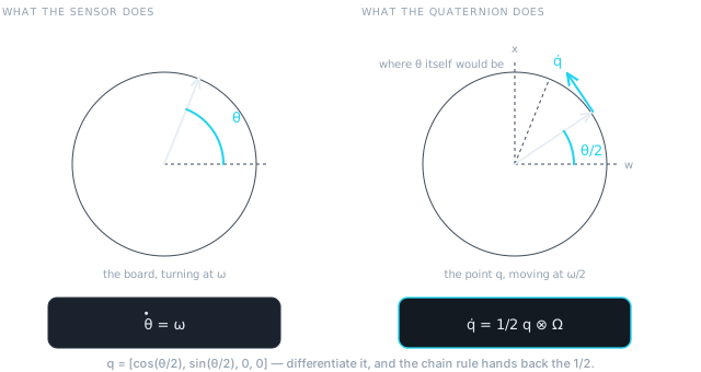Figure 2 — The same rotation, twice. The board sweeps through θ; the quaternion sweeps through θ/2, so it travels at half the rate. Differentiating the half angle is the whole origin of the factor.

What does the multiplication actually do?

The example also gives us a useful geometric interpretation.

The current quaternion $q$ describes where we are on the space of possible orientations.

The angular velocity describes how fast we are rotating.

The product

$$q\otimes\Omega$$

therefore produces the direction in which the current quaternion must move in quaternion space.

It is useful to think of it as a tangent vector to the quaternion trajectory.

The multiplication does not simply “rotate the angular velocity vector into the world frame.” A direct frame transformation would instead be

$$\omega_{world} = q\otimes\Omega_{body}\otimes q^*$$

where $q^*$ is the conjugate quaternion.

The propagation equation has a different purpose: it combines the current orientation with the body-frame angular velocity to calculate the rate of change of the orientation itself.

This distinction becomes important when implementing an estimator.

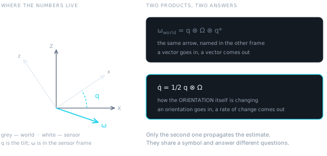Figure 3 — Both products contain q and Ω, and they answer different questions. Only the lower one propagates the estimate.

Both appear in the firmware, a few lines apart, doing unrelated jobs.

Numerical Quaternion Integration

Once the quaternion derivative has been calculated, we can integrate it just as we integrated angular velocity in the previous experiment.

Using a simple Euler integration step,

$$q_{k+1}=q_k+\dot q_k\Delta t$$

or

$$q_{k+1} = q_k+ \frac{1}{2} q_k\otimes\Omega_k\Delta t$$

Because numerical integration introduces small errors, the resulting quaternion may slowly move away from unit length.

We therefore normalize it after each update:

$$q_{k+1} \leftarrow \frac{q_{k+1}}{\|q_{k+1}\|}$$

That costs one square root per sample. Across the 27-second sweep recorded further down, the quaternion never left unit length by more than 0.00026.

This gives us a complete quaternion-based gyroscope integrator.

However, just like the Euler-angle implementation from Experiment #008, pure gyroscope integration will drift.

We therefore need an external reference.

Gravity as an Orientation Reference

When the sensor is stationary, the accelerometer measures the direction of gravity.

After normalization, the accelerometer measurement can be treated as a unit vector:

$$\mathbf{a}= \frac{\mathbf{a}_{raw}} {\|\mathbf{a}_{raw}\|}$$

Our quaternion represents the estimated orientation of the sensor.

From this orientation, we can calculate what the gravity direction should look like in the sensor frame.

For this experiment, gravity is defined in the world frame as

$$\mathbf{g}_{world}= \begin{bmatrix} 0\\ 0\\ 1 \end{bmatrix}$$

Since our quaternion represents body-to-world orientation, we use its conjugate to transform the world gravity vector into the body frame:

$$\mathbf{g}_{estimated} = q^* \mathbf{g}_{world}$$

In the implementation, this transformation is performed using the quaternion vector-rotation operation.

We now have two vectors:

• $\mathbf{a}$ — measured gravity direction,
• $\mathbf{g}_{estimated}$ — gravity direction predicted by our orientation estimate.

If the orientation estimate is correct, the two vectors should coincide.

Turning the Gravity Difference into a Feedback Signal

The difference between these two vectors gives us information about how the orientation estimate is wrong.

We calculate the error vector using the cross product:

$$\mathbf{e} = \mathbf{a} \times \mathbf{g}_{estimated}$$

The direction of $\mathbf{e}$ is perpendicular to both vectors and therefore gives the axis around which the estimated orientation should be corrected.

The magnitude is

$$\|\mathbf{e}\| = \sin(\theta_e)$$

where $\theta_e$ is the angle between the measured and estimated gravity vectors.

For small errors,

$$\sin(\theta_e)\approx\theta_e$$

Thus, the cross product gives us a convenient rotational error signal.

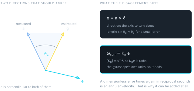Figure 4 — The cross product gives both halves of a correction at once: an axis to turn about, and a length that is the error angle in radians while the error is small.

This is a proportional controller

At this point the structure of the estimator becomes much clearer.

We have:

• a reference: measured gravity,
• a state: quaternion orientation,
• an estimated output: gravity calculated from the quaternion,
• an error: cross product of measured and estimated gravity,
• a controller: proportional gain $K_p$,
• an actuator-like control input: angular-velocity correction,
• an integrator: quaternion propagation.

The correction is

$$\boldsymbol{\omega}_{correction} = K_p\mathbf{e}$$

The corrected gyroscope measurement is then

$$\boldsymbol{\omega}_{corrected} = \boldsymbol{\omega}_{gyro} + K_p\mathbf{e}$$

The corrected angular velocity is used by the quaternion integrator.

This creates a closed feedback loop.

The important point is that we are not directly “moving the quaternion toward the accelerometer quaternion.”

Instead, the proportional controller generates an angular velocity correction. That correction changes the quaternion through the normal physical relationship between angular velocity and orientation.

This makes the estimator behave like a rotational feedback controller.

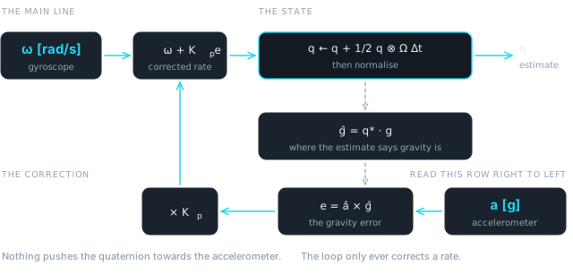Figure 5 — The whole estimator. The only path into the quaternion is the integrator, and the only thing the accelerometer does is bend a rate.

Why can we add the correction to angular velocity?

There is also a useful dimensional interpretation.

Both $\mathbf{a}$ and $\mathbf{g}_{estimated}$ are normalized, so their cross product is dimensionless. For small angles, its magnitude is approximately the angular error in radians.

Therefore $K_p$ must have units of inverse seconds:

$$[K_p]=s^{-1}$$

Consequently,

$$[K_p\mathbf{e}]=rad/s,$$

which has the same units as the gyroscope measurement.

So the correction is dimensionally consistent with angular velocity.

The Complete Quaternion Complementary Filter

The complete update sequence is therefore:

1. Normalize the accelerometer.
2. Calculate the gravity direction predicted by the current quaternion.
3. Calculate the gravity error using the cross product.
4. Multiply the error by $K_p$.
5. Add the correction to the gyroscope measurement.
6. Integrate the quaternion using the corrected angular velocity.
7. Normalize the quaternion.

In compact form:

$$\mathbf{a}_n= \frac{\mathbf{a}} {\|\mathbf{a}\|}$$ $$\mathbf{g}_{estimated} = R(q)^T\mathbf{g}_{world}$$ $$\mathbf{e} = \mathbf{a}_n\times\mathbf{g}_{estimated}$$ $$\boldsymbol{\omega}_{corrected} = \boldsymbol{\omega}_{gyro} + K_p\mathbf{e}$$

and finally

$$q_{k+1} = normalize \left( q_k+ \frac{1}{2} q_k\otimes \Omega_{corrected} \Delta t \right)$$

There is not a trigonometric function anywhere in that sequence. ahrs_update() and quaternion_integrate() in the firmware are the seven steps written out, and both are in ahrs.c and quaternion.c in the release linked at the foot of this article.

Two details decide whether the implementation works. The gyroscope channels in this firmware are in degrees per second, so the conversion to radians per second happens once, at the call site — getting it wrong scales the whole correction by 57. And ahrs_init() seeds the starting quaternion from an averaged accelerometer attitude once the zero-offset estimator reports ready, so a recording does not open with a convergence transient that has nothing to do with the experiment.

Experimental Convergence

The experimental setup is the same hardware and measurement environment used in the previous MPU6050 experiments. The details are therefore not repeated here. The sensor runs at 1 kHz with its internal low-pass filter at about 21 Hz, ±2 g and ±250 °/s, and EmbedStudio read the firmware’s own estimator state over SWD at roughly 127 samples per second.

One thing about the firmware does matter for what follows. The estimator is instantiated three times, with $K_p$ = 0.1, 1 and 10, and all three run over the same samples. They share nothing but their inputs, so every comparison below is between estimates of the same motion rather than between separate recordings. On the 168 MHz Cortex-M4 the whole signal-processing chain — three quaternion estimators, six complementary filters from #009 and everything else — measured 81 µs per sample against a 1000 µs loop. The sensor read over I²C remains the expensive part, at 414 µs.

To observe the convergence behavior, the orientation estimate was intentionally reset to an incorrect orientation while the board remained stationary. On request, every estimator is re-initialised as though gravity pointed along the sensor’s +Y axis. The board was lying still and level, so that is a 90° roll away from the truth, and it puts the quaternion at $[0.7071, 0.7071, 0, 0]$ — the worked value from figure 1.

The estimator then started from this incorrect state and used the accelerometer-derived gravity direction as its reference. The gyroscope reads nothing, because nothing is moving. Everything that happens next is the accelerometer pulling the estimate back.

Quaternion convergence

The first experiment records all four quaternion components:

$$q_w,\quad q_x,\quad q_y,\quad q_z$$

Immediately after the reset, the quaternion represents the incorrect orientation.

As the feedback loop operates, the gravity error generates an angular-velocity correction. The quaternion consequently moves toward an orientation consistent with the measured gravity direction.

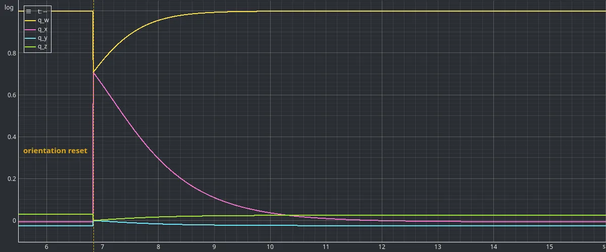Figure 6 — The Kp = 1 estimator, reset at 6.835 s and recovering. The step is instantaneous and the return is not: it is a first-order decay driven entirely by the gravity error.

The step into the wrong orientation is instantaneous and the return is not. The scalar and X components leave 1 and 0 together, and come back together over about four seconds, while Y and Z stay near zero throughout — the error was a pure roll and the correction stays one too.

Gravity-vector convergence

An even more direct way to observe the convergence is to compare:

$$\mathbf{a}$$

and

$$\mathbf{g}_{estimated}$$

The three components of the measured and estimated gravity vectors should converge toward each other.

The corresponding angular error can be calculated as

$$\theta_e = \arccos \left( \mathbf{a}\cdot \mathbf{g}_{estimated} \right)$$

This provides a scalar measure of the remaining orientation error that is directly related to the feedback signal.

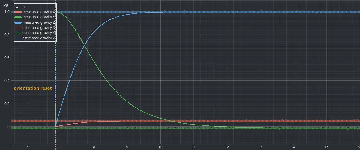Figure 7 — The same event as figure 6, in the loop’s own error terms. The thick bands are the measured direction and the sharp curves are the estimate; they coincide before the reset and again afterwards. The accelerometer is recorded in g rather than as a unit vector, so it is drawn scaled by 1/|a| = 0.976243, the median magnitude measured in this capture.

The measured direction never moves — the board is still. The estimated direction starts 90° away and walks back onto it. That walk is the entire mechanism of the filter, and its speed is the only thing the gain controls.

Influence of the Proportional Gain

The proportional gain determines how strongly the accelerometer error influences the estimated angular velocity.

We tested three values:

$$K_p=0.1,\quad 1,\quad 10$$

A low gain produces a relatively slow correction. The estimator relies more heavily on the gyroscope and takes longer to eliminate an orientation error.

Increasing the gain makes the correction stronger and therefore accelerates convergence.

The measured gravity-angle error provides a particularly useful way of comparing this behavior.

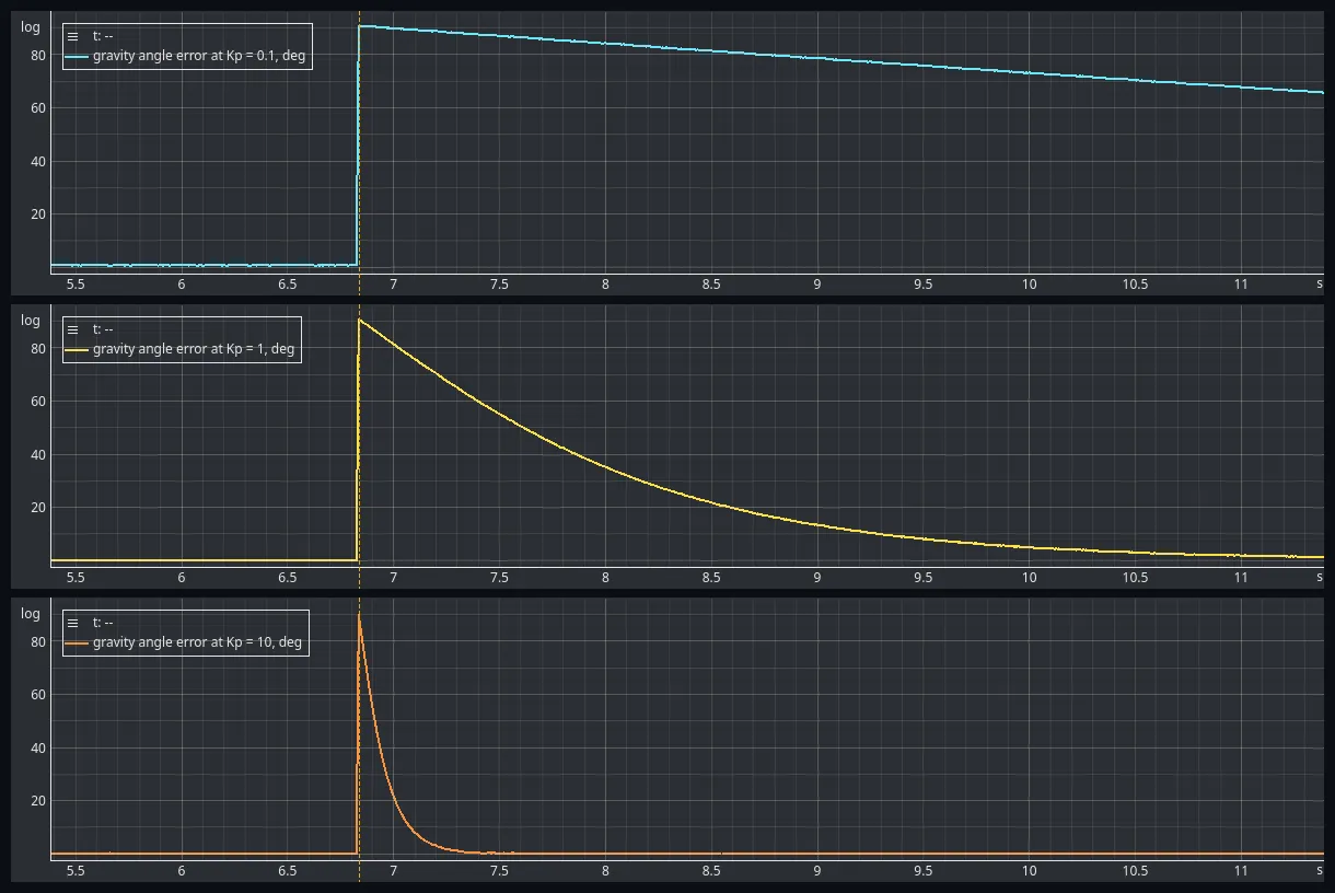Figure 8 — One gain per panel, and the same axes in all three. The dashed line is the reset. At Kp = 0.1 the error has barely started to come down when the frame ends; at Kp = 1 it is finished inside it; at Kp = 10 it is over in the first tenth of the panel. Ten times the gain, ten times faster, twice over.

The three curves are the same curve at three speeds. Fitting the decay over the stretch from 30° to 3°, where the error is small enough for the linear approximation to hold, gives a time constant of 9.86 s at $K_p$ = 0.1, 0.9925 s at $K_p$ = 1 and 0.0996 s at $K_p$ = 10.

The loop’s time constant is $1/K_p$ seconds. That is what the gain means, and it is a far more useful way to choose one than picking a number and watching what happens — the same argument that made τ rather than α the quantity to choose in experiment #009.

Both this fit and the settling times are taken from the whole recording rather than from the six seconds drawn above; the $K_p$ = 0.1 decay runs on for another three quarters of a minute past the right-hand edge of its panel. The capture is published with this article, so the numbers can be checked. Measured as time to come back from 90.7° to under 1°, the three gains took 0.47 s, 4.8 s and 47.8 s. The early part of each decay is slightly slower than the fit predicts, because the error signal is $\sin\theta_e$ and at 90° that is 1 rather than 1.57.

Convergence speed is only half of what the gain decides. The other half is what the loop is still carrying once the transient is long finished.

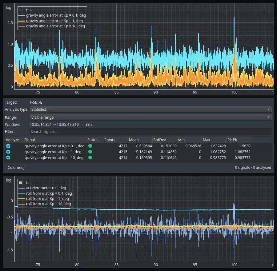Figure 9 — Over 33 settled seconds the angle between measured and estimated gravity averages 0.640° at Kp = 0.1, 0.182° at Kp = 1 and 0.170° at Kp = 10. Below, the same three estimators’ roll: the low gain sits about half a degree off the accelerometer’s mean and the other two sit on it. Kp = 1 is drawn 3 px wide under Kp = 10 at 1 px, because the two otherwise coincide.

The low gain leaves a standing error and the other two do not. This is not noise, and it is not an unfinished transient — the loop has been settled for a minute by this point. The gyroscope has a residual bias, the loop can only cancel it by producing an equal and opposite correction, and the only way it can produce a correction is to hold a non-zero error. The error it settles at is the bias divided by the gain, which is what 0.640° against 0.182° shows.

However, the accelerometer is not a perfect gravity sensor during motion. Linear acceleration, vibration and sensor noise can all appear as errors in the gravity measurement.

Consequently, increasing $K_p$ also increases the influence of these disturbances on the orientation estimate. The comparison of $K_p=0.1$, $1$ and $10$ therefore sits on the fundamental trade-off of the proportional feedback approach:

• low gain → slower correction and greater reliance on the gyroscope,
• high gain → faster correction but stronger sensitivity to accelerometer disturbances.

Neither capture here measures that second line. Both recordings are of a board that is either stationary or turning, so the accelerometer is never reporting anything but gravity, and the three gains’ settled standard deviations differ by less than a twentieth of a degree. Experiment #009 measured the disturbance directly, by translating the board without turning it. Take that half of the trade-off from there and the time constant from here.

Behavior Around ±90° Pitch

One of the main motivations for introducing quaternions is the singularity of Euler-angle representation around ±90° pitch.

We therefore repeated the orientation experiment while sweeping the sensor through this region. The board was pitched past vertical twice in each direction, with the estimator running at $K_p$ = 1.

The quaternion representation itself remains continuous during the motion.

The quaternion components

$$\quad q_x,\quad q_y,\quad q_z$$

do not encounter a singularity at ±90° pitch.

Euler angles can still be calculated from the quaternion for visualization:

$$(\phi,\theta,\psi) = f(q)$$

but the conversion back to Euler angles necessarily inherits the limitations of the Euler representation.

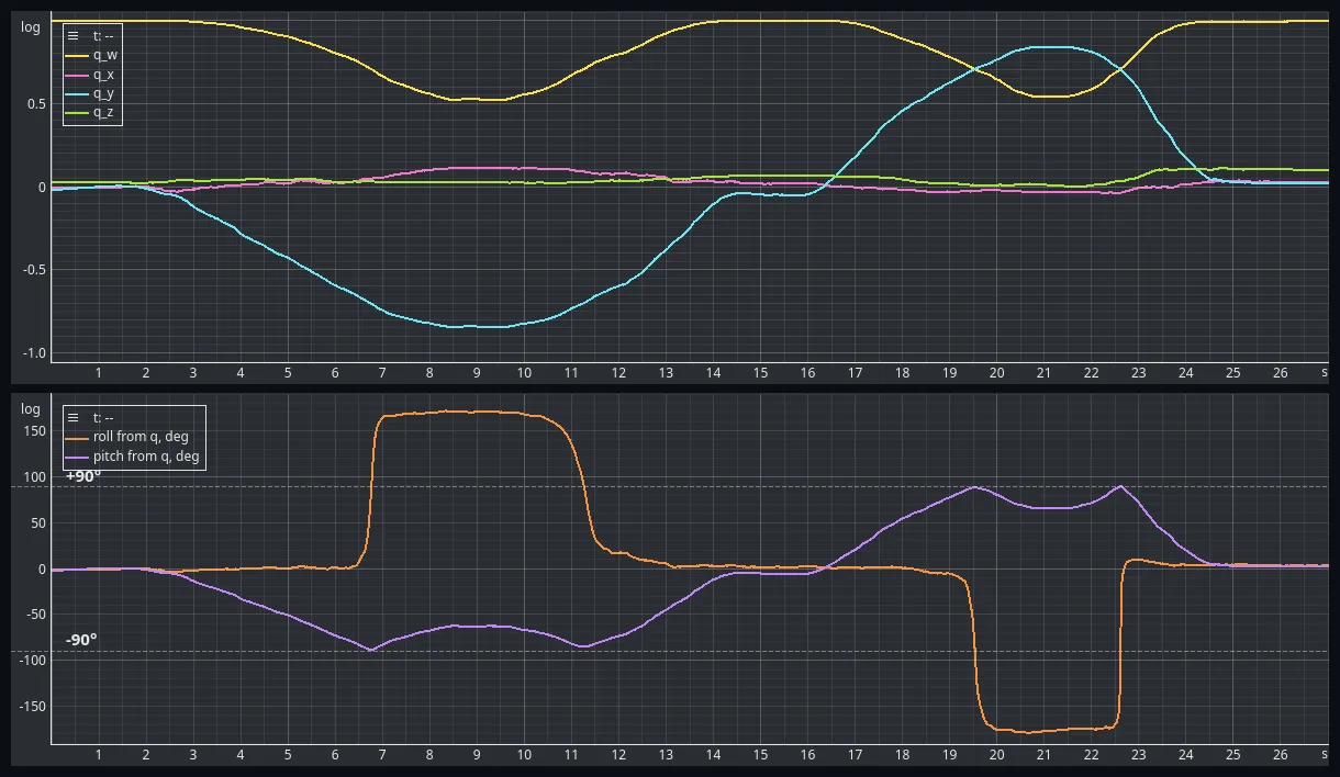Figure 10 — One estimator, two readings of it. The upper panel is the state the filter actually keeps; the lower panel is that state converted to Euler angles for display. Nothing happens to the quaternion at ±90° of pitch. Everything happens to the angles.

The sharpest instance is at 22.58 s. Over the next 62 ms:

• no quaternion component changes by more than 0.0143;
• the roll computed from it moves from −156.5° to −16.9°, a swing of 139.6°;
• the physical orientation — the angle between the two quaternions — changes by 3.17°.

Across the whole recording, the largest single-sample change in any quaternion component is 0.0051, and it happens outside the near-vertical region, not inside it. The largest single-sample change in Euler roll is 36.4°, and it happens at 89.5° of pitch. The quaternion is calmest exactly where the angles are wildest.

This distinction is important.

The quaternion estimator does not become singular simply because the resulting Euler-angle representation becomes difficult to interpret. None of this makes the Euler angles wrong either: they are a correct reading of a correct estimate, and a bad coordinate system near vertical.

Quaternions therefore provide a much better internal representation for the orientation estimator, while Euler angles remain useful as a human-readable visualization.

Discussion and Limitations

The experiment demonstrates that the quaternion representation provides a convenient way to propagate orientation using gyroscope measurements while avoiding the singularity inherent to Euler angles.

The gravity-feedback mechanism also fits naturally into the quaternion formulation.

However, several limitations remain.

Accelerometer corrections only constrain two degrees of freedom

Gravity defines a direction, not a complete orientation.

Rotating the sensor around the gravity axis does not change the measured gravity vector.

Therefore the accelerometer can correct roll and pitch, but it cannot determine absolute yaw.

Yaw remains dependent on the gyroscope integration and will therefore continue to drift. This experiment leaves that axis exactly as experiment #008 left it.

Linear acceleration affects the gravity reference

The accelerometer measures specific force rather than gravity alone.

During translational acceleration, the measured vector is no longer equal to the gravity vector. The feedback controller can therefore interpret linear acceleration as an orientation error.

This is the fundamental limitation of using an accelerometer as a gravity reference.

Gyroscope bias remains

The proportional feedback can correct orientation errors caused by gyroscope drift as long as those errors are observable through gravity.

However, it does not explicitly estimate the gyroscope bias. It suppresses the effect of the bias by dividing it by the gain, and the leftover is the standing error measured above: 0.640° at $K_p$ = 0.1 against 0.182° at $K_p$ = 1.

This motivates the next step.

Next: Mahony AHRS

The proportional gravity correction already has the structure of a feedback controller.

The next logical improvement is to add an integral term.

An integral controller can accumulate the persistent orientation error caused by gyroscope bias and use it to estimate and compensate that bias.

This leads to the Mahony attitude filter.

In the next experiment, we will extend the proportional quaternion feedback developed here with this integral term and investigate whether it can reduce the long-term gyroscope drift observed in the previous experiments.

Conclusion

In this experiment, we replaced Euler angles with quaternions as the internal representation of orientation.

More importantly, we derived the quaternion propagation equation rather than treating it as a black box.

Starting with the familiar relationship

$$\dot{\theta}=\omega$$

we showed that the half-angle representation of a quaternion naturally leads to

$$\dot q=\frac{1}{2}q\otimes\Omega$$

We then used the accelerometer to obtain an independent gravity reference and constructed a proportional feedback loop that generates an angular-velocity correction from the difference between measured and estimated gravity.

The resulting estimator combines:

• quaternion-based orientation propagation,
• gyroscope measurements for short-term dynamics,
• accelerometer measurements for long-term gravity reference,
• and proportional feedback for correcting orientation drift.

The experiments with different proportional gains put a number on the gain: the loop’s time constant is $1/K_p$ seconds, measured at 9.86, 0.9925 and 0.0996 s across two decades, and the standing error it leaves behind is the gyroscope bias divided by that same gain. The ±90° pitch experiment shows why quaternions are preferable as the internal orientation representation — a component moved by 0.0143 while the roll read from it moved 139.6°.

The next step is to add integral feedback and allow the estimator to explicitly track gyroscope bias, leading to a Mahony-style AHRS.

Experiment data

The raw datasets used in this experiment are publicly available in the EmbedStudio Experiments repository.

The dataset contains:

• a 106-second stationary recording carrying the orientation reset, used for the convergence figures and every gain comparison;
• a 27-second hand-held sweep through ±90° of pitch, in each direction twice.

Both captures carry all three estimators’ gravity error, error vector and estimated gravity direction, the Euler angles derived from each of them, the raw accelerometer and gyroscope, the τ = 500 ms complementary filter from experiment #009 for comparison, the die temperature and two firmware timing counters. The quaternion itself is recorded for the $K_p$ = 1 estimator only.

The gain is not a channel. It is a compile-time constant, and the mapping from estimator index to gain is in the manifest.

All datasets are provided as HDF5 files and can be downloaded and opened with EmbedStudio or another compatible HDF5 tool.