What Does a Complementary Filter Actually Fix?

The previous three experiments left us with two attitude sensors, each useless in a different way.

Experiment #006 estimated roll and pitch from gravity. It never walks away from the truth. But every sample carries noise, and any movement of the board is indistinguishable from a change of inclination. Experiment #007 showed that the roll half of that estimate falls apart as pitch approaches ±90°.

Experiment #008 integrated the gyroscope instead. That estimate is smooth, it handles fast rotation, and it passes straight through orientations where the accelerometer gives up. But it drifts, and it has no idea where it started.

The failures are opposite. The accelerometer is wrong in the short term and right in the long term; the gyroscope is the other way round.

The complementary filter is the cheapest way to exploit that. This experiment measures what it actually buys.

The acquisition configuration is unchanged from the previous experiments — the sensor runs at 1 kHz with its internal low-pass filter at about 21 Hz, ±2 g and ±250 °/s. EmbedStudio read the firmware’s own attitude variables over SWD at roughly 200 samples per second.

How the Complementary Filter Works

One line does the whole thing:

$$\theta_k = \alpha\,(\theta_{k-1} + \omega_k\,\Delta t) + (1 - \alpha)\,\theta_{\mathrm{acc}}$$

The first term is the gyroscope answer — the previous output advanced by the measured rotation. The second is the accelerometer answer. $\alpha$ decides how much of each survives.

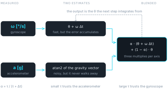Figure 1 — The two estimates and the blend. The output feeds back into the integration term, which is what makes the accelerometer correction compound instead of being applied once.

Implementing It on the Target

The filter itself is five lines:

void ahrs_complementary_filter(const ahrs_attitude_t* const accel_attitude,
        const vector_3f_t* const gyro, vector_3f_t* const attitude,
        const float alpha, const float dt_s)
{
    attitude->x = alpha * (attitude->x + gyro->x * dt_s)
            + (1.0f - alpha) * accel_attitude->roll;
    attitude->y = alpha * (attitude->y + gyro->y * dt_s)
            + (1.0f - alpha) * accel_attitude->pitch;
    attitude->z += gyro->z * dt_s;
}

Where that alpha comes from is the next section. Three things around the five lines matter more than the five lines do.

Seed all the accumulators together, and seed them from an average. Before the first blend, roll and pitch are set from the accelerometer and yaw to zero. One accelerometer sample carries the 0.056° of noise measured further down, so the firmware averages 100 of them, and only starts once the gyroscope zero-offset estimator reports ready. The integrator and all six filters are released at the same instant from the same value.

Feed the filter the gyroscope’s calibrated rate, not the raw one. The bias removed in experiment #003 is what makes the gyroscope term worth blending in at all.

Handle the wrap, or avoid it. The blend is arithmetic on two floats and knows nothing about angles. Before combining, wrap the difference $\theta_{\mathrm{acc}} - \theta$ into ±180° and add the correction to $\theta$, or work in a representation that does not wrap. The reference firmware here does neither, deliberately — it is a measurement rig, and figure 8 below is what that choice looks like.

Picking the Time Constant

Written as a weighted average the filter invites you to read $\alpha$ as “how much I trust the gyroscope”. That reading is not wrong, but it is not useful for choosing a number. $\alpha = 0.98$ means nothing on its own; it means something different at 1 kHz than at 100 Hz.

The quantity with physical meaning is the time constant:

$$\alpha = \frac{\tau}{\tau + \Delta t}$$

$\tau$ is how long the accelerometer takes to pull the estimate back towards gravity. $\Delta t$ is the sample interval, and the loop here runs at 1 kHz, so it is 1 ms. Pick $\tau$ in milliseconds, compute $\alpha$ from it, and the filter keeps behaving the same way if the loop rate changes.

Compute it once, at startup. The firmware does it as alpha[i] = tau_ms[i] / (tau_ms[i] + LOOP_TIME_MS), with LOOP_TIME_MS equal to 1, for six time constants:

$\tau$	$\alpha$ at $\Delta t$ = 1 ms
10 ms	0.909091
50 ms	0.980392
100 ms	0.990099
500 ms	0.998004
1000 ms	0.999001
5000 ms	0.999800

Note that the nominal interval goes into $\alpha$ while the measured one is what the filter integrates with. Experiment #004 put the real interval at 1.0009 ms, so every time constant here is 0.09 % longer than its label. That is below anything this experiment can see, but it is the kind of shortcut worth knowing you took.

All six run at once on the same samples, so every comparison below is between estimates of the same motion, not between two recordings. The five-minute stationary recording is the exception — it was taken before the last two were added, and carries the first four.

Yaw is not filtered. The accelerometer measures the direction of gravity, and rotation about gravity does not change it. There is nothing to blend with, so the filter leaves that axis exactly as experiment #008 left it. Everything below is about roll and pitch.

What It Costs to Run

The claim that a complementary filter is cheap gets repeated a lot, so it is worth a number.

The firmware already times its own signal-processing block with the DWT cycle counter from experiment #004, and EmbedStudio plots that counter beside the attitude channels. With six filters running, the whole chain measured a median of 45 µs per sample on a 168 MHz Cortex-M4. That is calibration, gravity magnitude, the zero-offset estimator, atan2 twice, the integration and all six blends together.

For scale, reading the sensor over I²C in the same loop takes 414 µs, and the loop has 1000 µs to work with. Every piece of arithmetic in the loop costs about a tenth of what it takes to fetch the samples it runs on. The filter is not the expensive part of anything.

Five Stationary Minutes

The board was set down and left alone for five minutes. Nothing moved, so every difference between the three estimates is error.

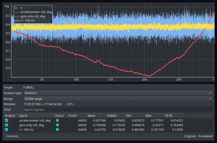Figure 2 — Roll, 297 s. The accelerometer (blue band) is noisy but centred; the gyroscope (red) is smooth but goes for a walk; the filter (yellow, τ = 100 ms) is both centred and smooth. The whole frame spans 0.85°.

The Analysis panel measures all three over the visible range at once, which is the comparison this experiment is about:

roll estimate	σ	peak-to-peak
accelerometer	0.056°	0.475°
gyroscope only	0.173°	0.742°
complementary, τ = 100 ms	0.016°	0.136°

The gyroscope’s σ is the largest of the three, and it is not noise. It is the slow wander of a curve that is individually smooth. Read the shape, not the number.

Pitch tells the same story with the volume turned up, because that axis had the larger residual bias on this board.

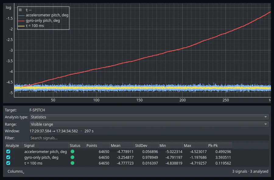Figure 3 — Pitch, the same 297 s. The gyroscope walks 3.59° away from where it started. Note the vertical span — this frame covers 4.4°, against 0.85° in figure 2, so the noise band that filled figure 2 is the flat line at the bottom here.

Over 297 s the gyroscope-only estimate moved +0.21° in roll and +3.59° in pitch. Every complementary filter ended within 0.06° in roll and 0.02° in pitch of where it started.

That is the first result, and it is the easy one. The accelerometer term has no memory, so there is nothing for a bias to accumulate into. Drift in roll and pitch is not reduced by the filter; it is gone.

The second result is the one the filter is usually not credited with:

τ	σ, roll	σ, pitch
accelerometer alone	0.056°	0.057°
10 ms	0.038°	0.039°
50 ms	0.021°	0.022°
100 ms	0.016°	0.016°
500 ms	0.009°	0.008°
gyroscope alone	0.004°	0.004°

The filter is a low-pass on the accelerometer as well as a high-pass on the gyroscope. At τ = 500 ms the stationary estimate is six to seven times quieter than the accelerometer it came from. The die temperature over the window moved only from 27.17 °C to 26.70 °C, so none of this is a thermal excursion.

The gain is not proportional to τ. Going from 10 ms to 100 ms cut the noise by 2.4; going from 100 ms to 500 ms cut it by another 1.7.

What Does the Time Constant Change?

A stationary board says nothing about response. The next recording is fourteen seconds of the board being turned about all three axes by hand and then put back down.

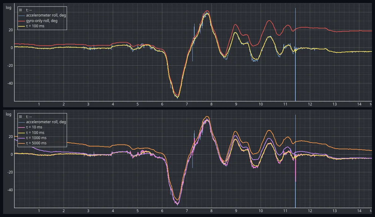Figure 4 — Fourteen seconds of hand motion. Above, the gyroscope-only estimate (red) ends 23.4° away from the accelerometer while the filter (yellow, τ = 100 ms) comes home. Below, the same motion through τ = 10, 100, 1000 and 5000 ms. The accelerometer trace leaves the frame once, at 11.41 s — that is figure 7.

When the board came to rest the gyroscope-only estimate was 23.4° wrong in roll and 7.7° wrong in pitch. The filters at τ = 10, 50 and 100 ms were within 0.01°, τ = 500 ms within 0.03° and τ = 1000 ms within 0.5°.

That 23° is worth being precise about, because it is not drift. Fourteen seconds at the residual bias measured in the previous section is 0.2°, a hundred times less. It is the axis-coupling error from experiment #008 — three Euler angles integrated independently, which is only valid near level. The filter did not correct a bias. It corrected an estimator that is wrong by construction, because the accelerometer term does not care why the integration went astray.

τ = 5000 ms behaves differently from the rest, and the lower panel shows why. It was still carrying an error from before the recording started, and it never caught up: at the end it was 10.2° out. The initial transient is a clean way to measure the correction time constant, since the error decays exponentially. Fitting it gives 1029 ms for the filter configured at 1000 and 5058 ms for the one configured at 5000. A second recording puts the latter at 4976 ms. The constants the firmware computes are the constants it gets.

The interesting part of the lower panel is what it does not show. Through the fast swing at 6.5 s, all four time constants are on top of each other.

A complementary filter does not delay real motion. The gyroscope path carries it, and the gyroscope path has no lag. What τ delays is the correction — the removal of an error the gyroscope path already has. That is why the noise figures above improve with τ and the tracking does not degrade.

The cost is on the other side of the same coin. A long τ is also slow to recover when the estimate is wrong for some other reason, which is what the last two sections are about.

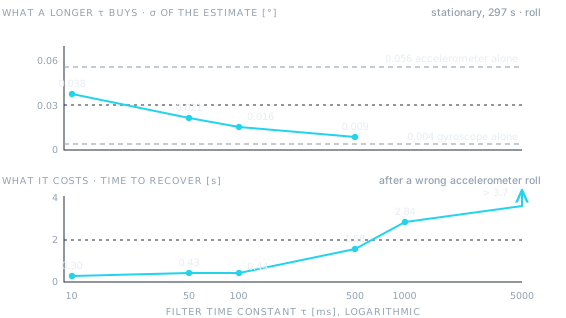Figure 5 — The trade-off, from the measurements in this article. Noise falls with τ and recovery time rises with it. The noise figures come from the five-minute stationary recording, the recovery figures from the high-pitch recording in the last section.

What Happens When You Shake It Without Turning It?

The accelerometer measures every acceleration, not just gravity:

$$a_{\mathrm{measured}} = g + a_{\mathrm{linear}}$$

Nothing in the filter can separate the two. To see how much that costs, the board was moved around by hand without being rotated.

The gyroscope says how well that worked: over the whole recording the integrated roll moved 2.4° peak-to-peak and the integrated pitch 3.1°. The board was barely turning.

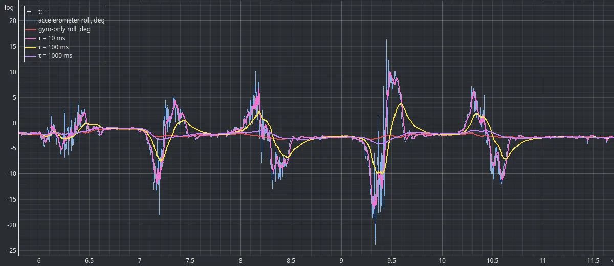Figure 6 — Translation, no rotation. The accelerometer roll swings 40° peak-to-peak while the gyroscope (red) says the board turned by two. The gyroscope trace is drawn shifted by −20.46°, the measured median gap between the two estimates, so its shape can be compared on this scale.

The accelerometer roll reached 21.2° away from its own median. Here is how much of that each filter passed through:

τ	worst excursion	σ over the window
accelerometer	21.2°	3.71°
10 ms	14.3°	3.39°
50 ms	10.3°	2.80°
100 ms	7.7°	2.20°
500 ms	3.0°	0.92°
1000 ms	1.8°	0.66°

A longer time constant attenuates the disturbance, and that is all it does. The filter never identifies linear acceleration and never rejects it; it averages it away, given enough time. Sustained acceleration — a vehicle accelerating for ten seconds — is not attenuated by any of these filters, because it is not a transient.

The motion recording from the previous section carries a second failure, and it is invisible at that figure’s scale. At 11.408 and 11.413 s two consecutive samples of accelerometer roll read −134.90° and +44.95°, between neighbours a few degrees from level. A sharp jolt can put the measured acceleration vector almost anywhere, and atan2 will faithfully report the angle of whatever it is given.

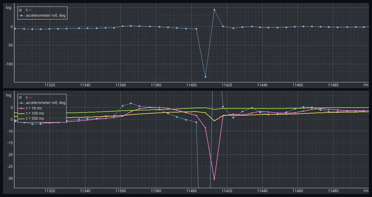Figure 7 — 200 ms of the same recording, at the only scale the glitch is visible at. Above, the accelerometer roll, one marker per sample. Below, the same window at the filters’ scale. In figure 4 this is one thin vertical line leaving the frame.

The τ = 10 ms filter dropped 27.1° below the sample before the glitch, and was back within 15 ms. τ = 100 ms moved 3.9° and took 56 ms to return. τ = 500 ms moved 0.6°, which is the width of its own noise.

If your filter is going to see impacts, a very short time constant is not a “fast” filter. It is an unprotected one.

Does It Fix the 90 Degree Problem?

Experiment #007 measured what happens to the roll estimate as pitch approaches ±90°. Roll is computed as $\mathrm{atan2}(a_y, a_z)$, and as the board approaches vertical both of those components shrink into the noise. The angle between two small noisy numbers is not a measurement.

That is a property of the accelerometer and of Euler angles, not of the gyroscope. So the question is whether blending in a sensor that is fine there rescues the estimate.

The board was pitched forward past vertical and brought back.

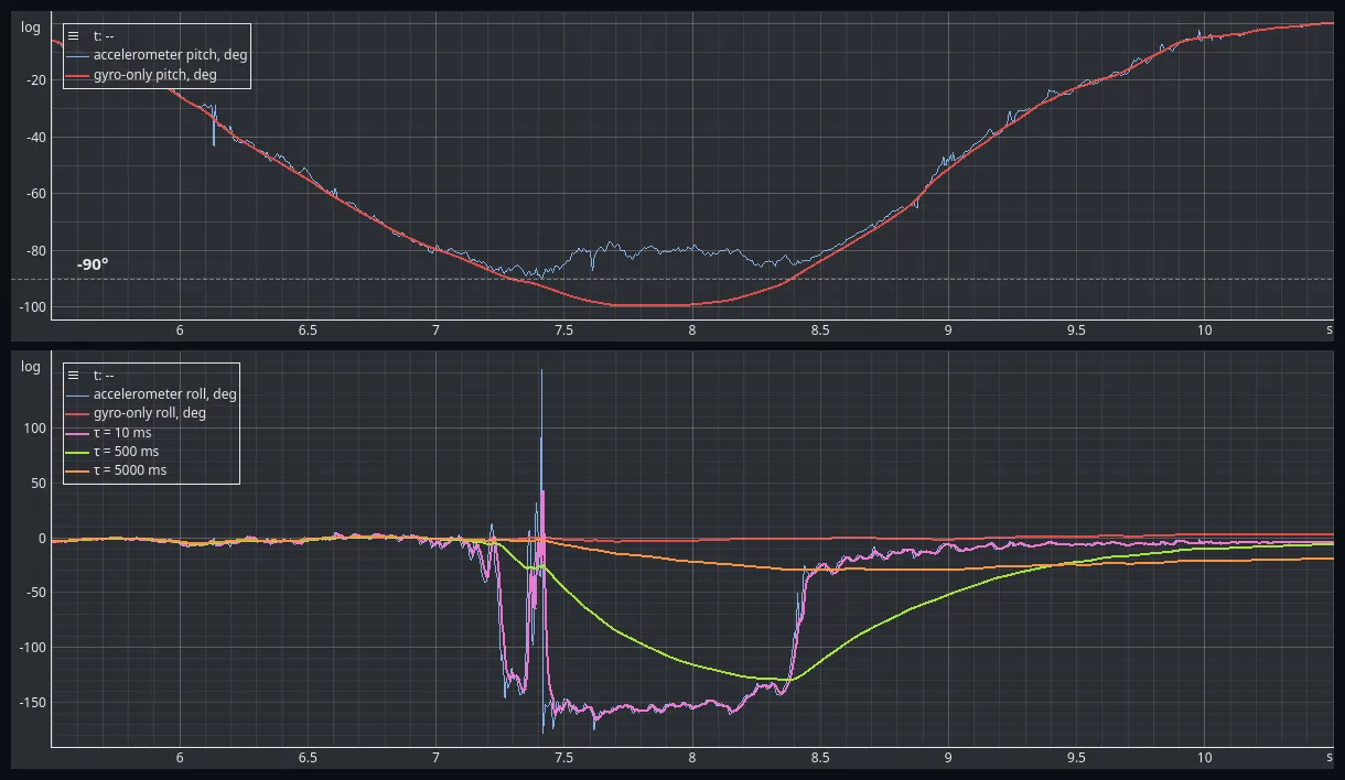Figure 8 — Pitched past vertical. Above, the accelerometer pitch stops at −89.8° and folds back while the integrated pitch passes through to −99.4°. Below, the roll estimates over the same seconds. The gyroscope (red) says the board barely rolled; the accelerometer (blue) says it rolled to −178°.

While the pitch was past 80° — 1.55 seconds, 236 samples — the accelerometer roll swung between +154° and −178°, and the gyroscope-integrated roll stayed inside ±3.6°. The gyroscope is right. The board was not rolling.

Every filter followed the accelerometer down:

τ	worst roll reported	time to recover afterwards
accelerometer	−178.0°	—
10 ms	−166.0°	0.30 s
50 ms	−159.2°	0.43 s
100 ms	−155.7°	0.44 s
500 ms	−130.0°	1.58 s
1000 ms	−98.1°	2.84 s
5000 ms	−29.6°	still 10.6° out after 3.68 s

A long time constant looks better in that table, and it is a trap. The 5000 ms filter is not more correct — it is slower. It was still 10.6° wrong three and a half seconds after the board came back to a normal attitude. It would have been just as wrong if the accelerometer had been telling the truth.

Sensor fusion and attitude representation are separate problems. The filter improves the quality of an estimate. It cannot repair a parameterisation that has stopped being able to express the answer.

There is one more thing in that lower panel, and it is a bug rather than a limitation. Between two consecutive samples the accelerometer roll reads +154.06° and then −162.95°. As orientations those are 43° apart. As numbers they are 317° apart, and the filter is doing arithmetic on numbers. Every blend across that wrap drags the output most of the way round the circle and back.

What Have We Learned?

What the complementary filter fixes

• Gyroscope drift in roll and pitch, completely. 3.59° of walk over five minutes became 0.02°.
• Accelerometer noise, by six to seven times at τ = 500 ms, and by 1.5 times even at τ = 10 ms.
• Errors the integration makes for reasons other than bias. The 23.4° of axis coupling measured here was removed without the filter knowing what it was.
• The cost of doing it. The whole signal-processing chain, six filters included, measured 45 µs against the 414 µs the sensor read costs in the same 1000 µs loop.

What it does not fix

• Linear acceleration. A hand-held translation put 21° into the accelerometer estimate, and a τ = 100 ms filter still passed 7.7° of it through. Attenuation is not rejection.
• The ±90° limitation. Roll from an accelerometer stops meaning anything near vertical, and blending does not restore information that was never measured. A long time constant hides the symptom for longer than the event lasts.
• Yaw. The accelerometer contributes nothing about rotation around gravity, so the filter leaves that axis untouched.
• Angle wrapping. The filter has no idea it is working with angles.

Conclusion

The complementary filter earns its reputation. One line of arithmetic per axis, no tuning matrix, no state covariance, no square roots. It removed every kind of long-term error the gyroscope had, and it made the accelerometer estimate several times quieter than the sensor it came from.

The time constant is the only thing to choose, and it is a genuine trade-off rather than a quality setting. Short means the estimate recovers quickly and carries accelerometer noise and impacts. Long means a clean estimate that stays wrong for a long time after something goes wrong. Between 50 ms and 500 ms covers most of what a hand-held board wants; 10 ms is barely a filter and 5000 ms is barely a correction.

What the experiment also shows is where the ceiling is. Two things still break the estimate: sustained linear acceleration, and the geometry of Euler angles near vertical. Neither is made better by blending harder. They need a different attitude representation, and a way to decide when the accelerometer should be believed at all.

That is where this journey goes next.

Experiment data

The raw datasets used in this experiment are publicly available in the EmbedStudio Experiments repository.

The dataset contains:

• the five-minute stationary recording used for the noise and drift figures;
• fourteen seconds of hand-held motion about all three axes, used for the time-constant comparison and the correction-time-constant fits;
• a translation-only recording in which the board is moved without being turned;
• a sweep past vertical in pitch, in which the accelerometer roll collapses.

Every capture carries the accelerometer attitude, the three integrated gyro angles, the output of every complementary filter, the filter constants themselves, the zero-offset estimator state, the die temperature and two firmware timing counters.

The five-minute recording carries four filters, not six. τ = 1000 ms and τ = 5000 ms were added to the firmware after it was taken, which is why the noise table above stops at 500 ms.

The EmbedStudio workspace the captures were recorded with is in the repository as well. It carries an extra Article figures dashboard whose views are the ones the screenshots above were taken from, so opening a capture with it puts the same plots on the screen.

All datasets are provided as HDF5 files and can be downloaded and opened with EmbedStudio or another compatible HDF5 tool.