See EmbedStudio in Action

Explore how EmbedStudio turns firmware variables into interactive development and analysis tools.

Overview

The whole workspace

Your Firmware, One Workspace

Combine plots, tables and other instruments into a workspace tailored to your project.
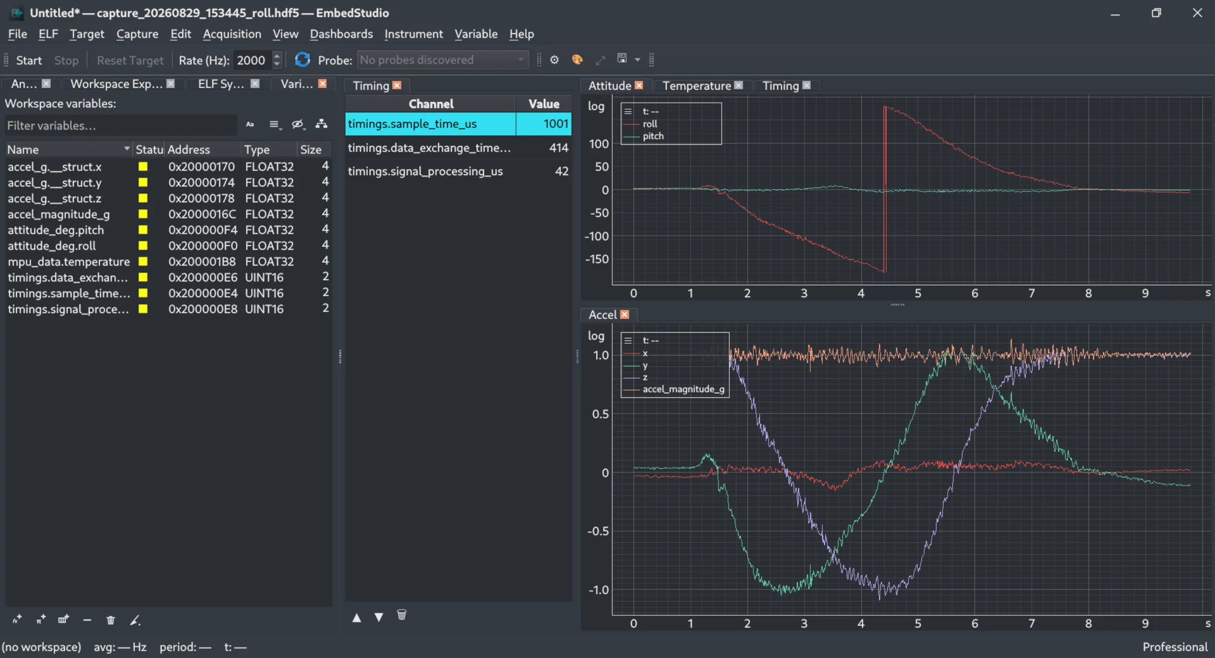
The EmbedStudio workspace: a variable explorer listing ELF symbols, a timing table, and two synchronized time plots of roll, pitch and accelerometer data
Variables

From ELF symbols to a workspace

Find Firmware Variables Automatically

Load your ELF file and browse the variables and type information discovered from its debug data.
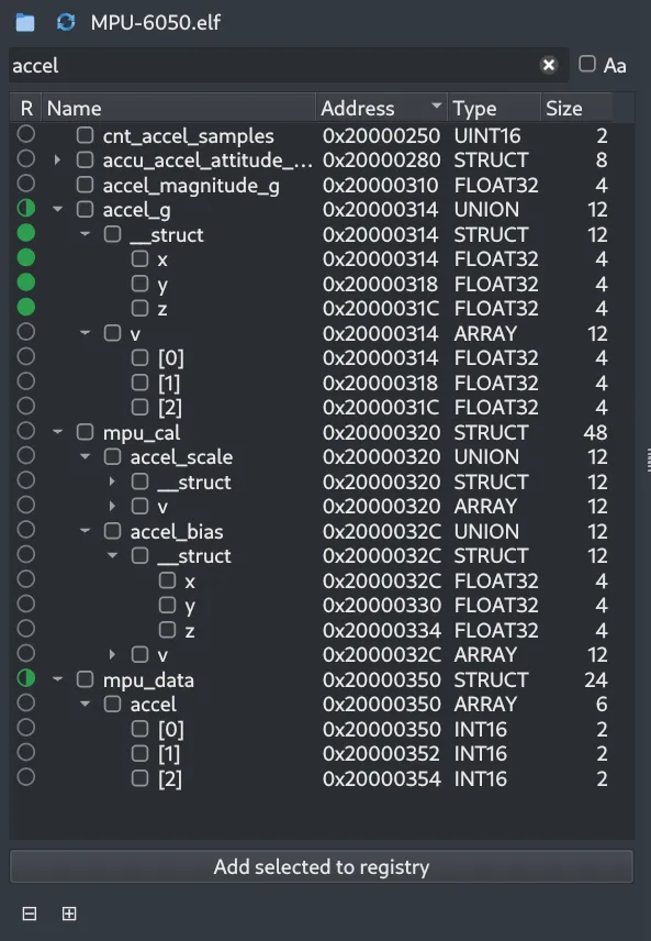
The ELF symbols browser filtered on "accel", showing a tree of structs, unions and arrays with each symbol’s address, type and size

Choose What to Acquire

Add variables from the ELF to your workspace and see each one’s address, type and size.
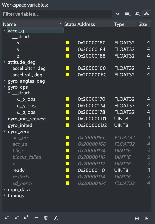
The workspace variables list showing the chosen variables grouped by struct, with their addresses, types and sizes
Instruments

Organize and inspect

Keep Dashboards Organized

See every dashboard and instrument in the workspace, and how many variables they need.
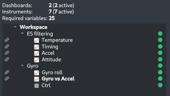
The workspace explorer showing two dashboards and the plot and table instruments each one contains

Inspect Values Directly

Use tables when numerical values are more useful than a graph.
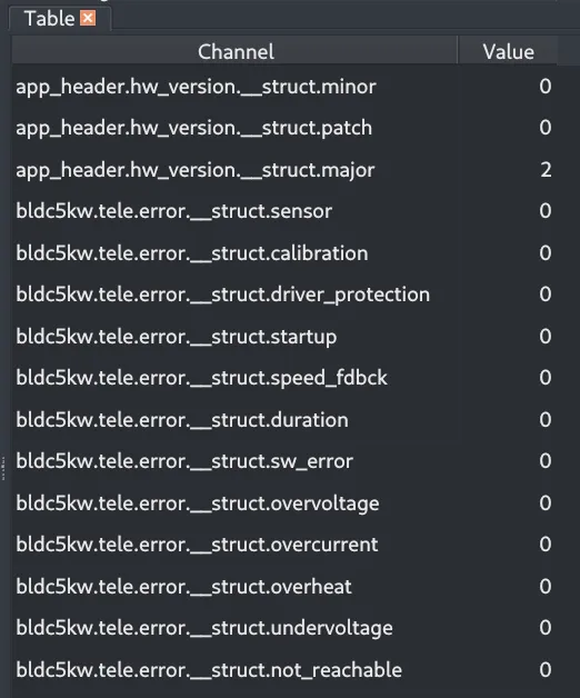
A table instrument listing firmware variables by name with their current values: hardware-version and error-flag fields, all reading 0 except a major version of 2
Visualization

Signals over time

Watch Signals in Real Time

Visualize firmware signals as they change and investigate system behavior without adding logging code.
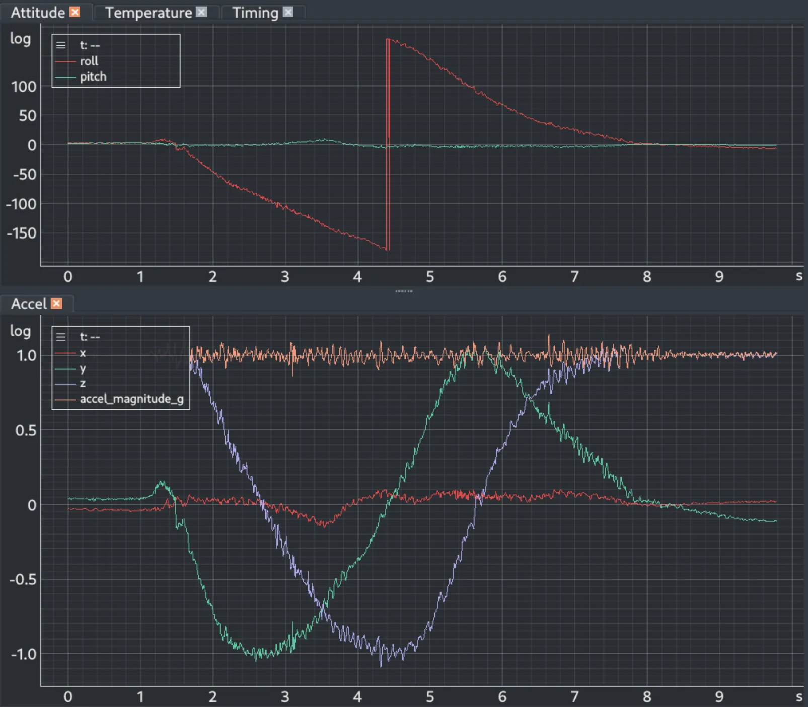
Two time plots: roll and pitch in degrees above, and the three accelerometer axes with their magnitude below

Style Every Trace

Choose each trace’s color, line style, width, marker and opacity, rename channels for one view, and reorder or hide them.
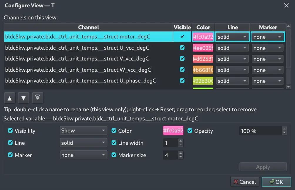
The Configure View dialog for a time plot: a table of channels with visibility, color, line style and marker, and below it controls for the selected variable’s color, opacity, line width and marker size
More instruments

Relations and states

Plot One Signal Against Another

Draw one variable against another instead of against time, for example the two channels of an encoder.
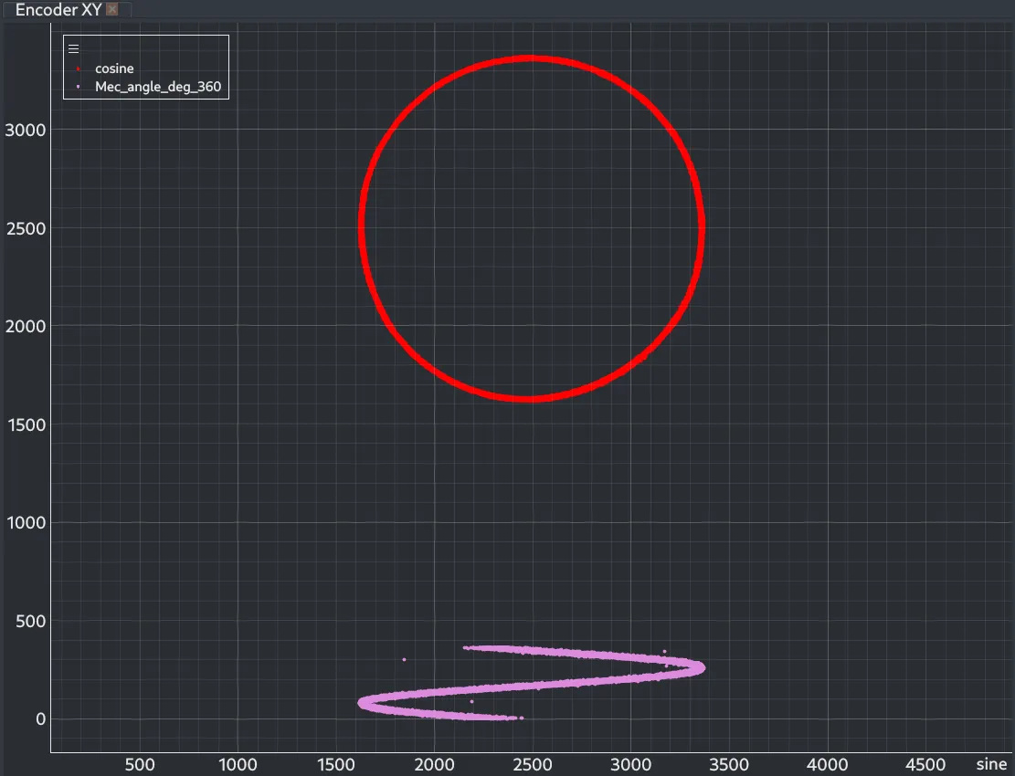
An XY plot of two encoder signals: the cosine against the sine traces a near-perfect circle, and a calculated angle against the sine draws a zig-zag below it

Follow States and Status Bits

Show flags, discrete values and booleans as rows on a timeline, lined up with a time plot above it.
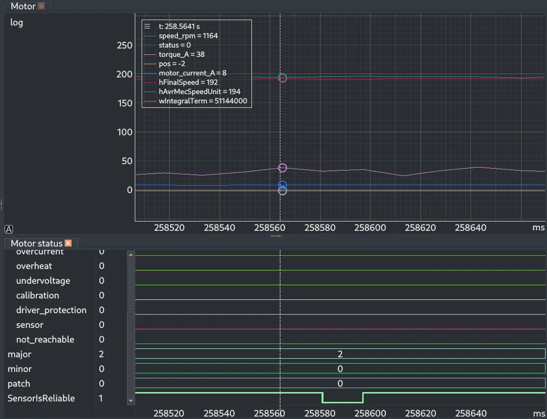
A time plot of motor speed, current and torque above a digital plot whose rows show status flags as flat lines, three numeric version fields and a boolean sensor signal that drops low briefly, with one cursor running through both
Measurement

Numbers from the signals

Measure What the Plot Shows

Place cursors on a plot and read the statistics of every signal between them: mean, deviation, extremes, RMS and integral.
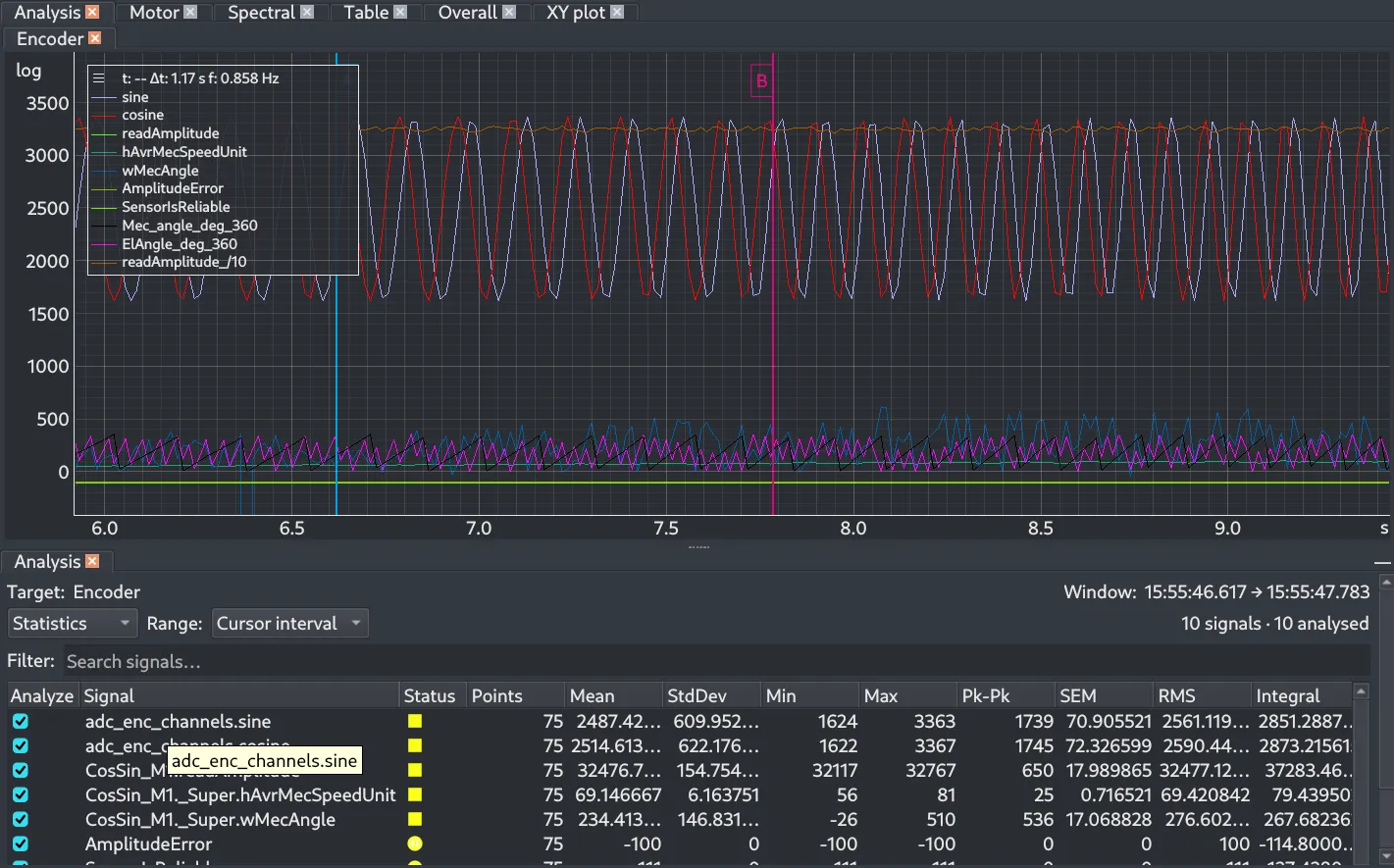
A time plot of encoder signals with two measurement cursors, above an analysis panel listing mean, standard deviation, minimum, maximum, peak-to-peak, SEM, RMS and integral for each signal over the cursor interval
Analysis

Frequency-domain analysis

Go Beyond Time-Domain Data

Use built-in analysis tools such as FFT to investigate the frequency content of acquired signals.
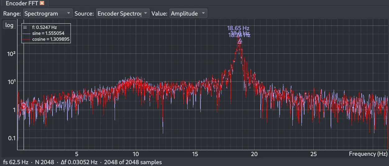
An FFT instrument showing the amplitude spectrum of an encoder’s sine and cosine channels on a log scale, with the strongest peaks marked near 18.7 Hz and the sampling rate, transform size and frequency resolution below

See Frequency Content Change Over Time

Use a spectrogram to follow how the frequency content of a signal evolves across an acquisition.
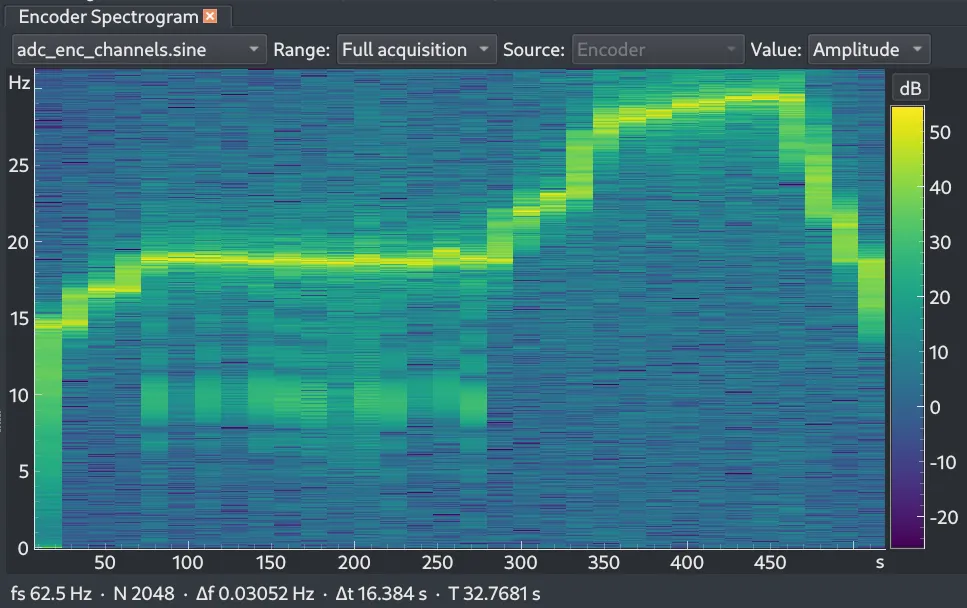
A spectrogram instrument: frequency in Hz on the vertical axis against time in seconds, colored by amplitude in dB, with a bright ridge that holds near 19 Hz and later climbs to about 29 Hz

Tune the Transform

Choose the window, size and overlap, the sample-rate handling and how amplitude is colored.
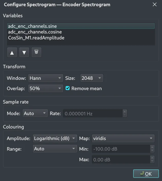
The Configure Spectrogram dialog: the list of variables, the transform window, size, overlap and mean removal, the sample-rate mode, and the amplitude scale, color map and range

From a Spectrogram Frame to Its Spectrum

Select a frame in the spectrogram and the FFT instrument shows the spectrum of that moment, with its peaks marked.
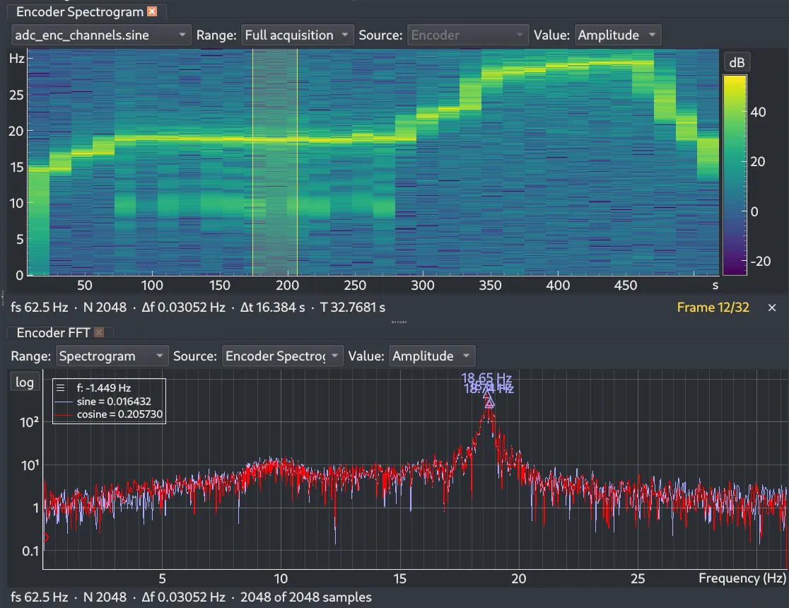
A spectrogram above an FFT instrument: one frame of the spectrogram is selected, and the FFT shows that frame’s amplitude spectrum with its strongest peaks marked
Calculated signals

Derive what you need

Create Derived Signals

Build calculated channels from acquired data to expose the information you actually need to investigate. As you type an expression, variable names are suggested from your registry.
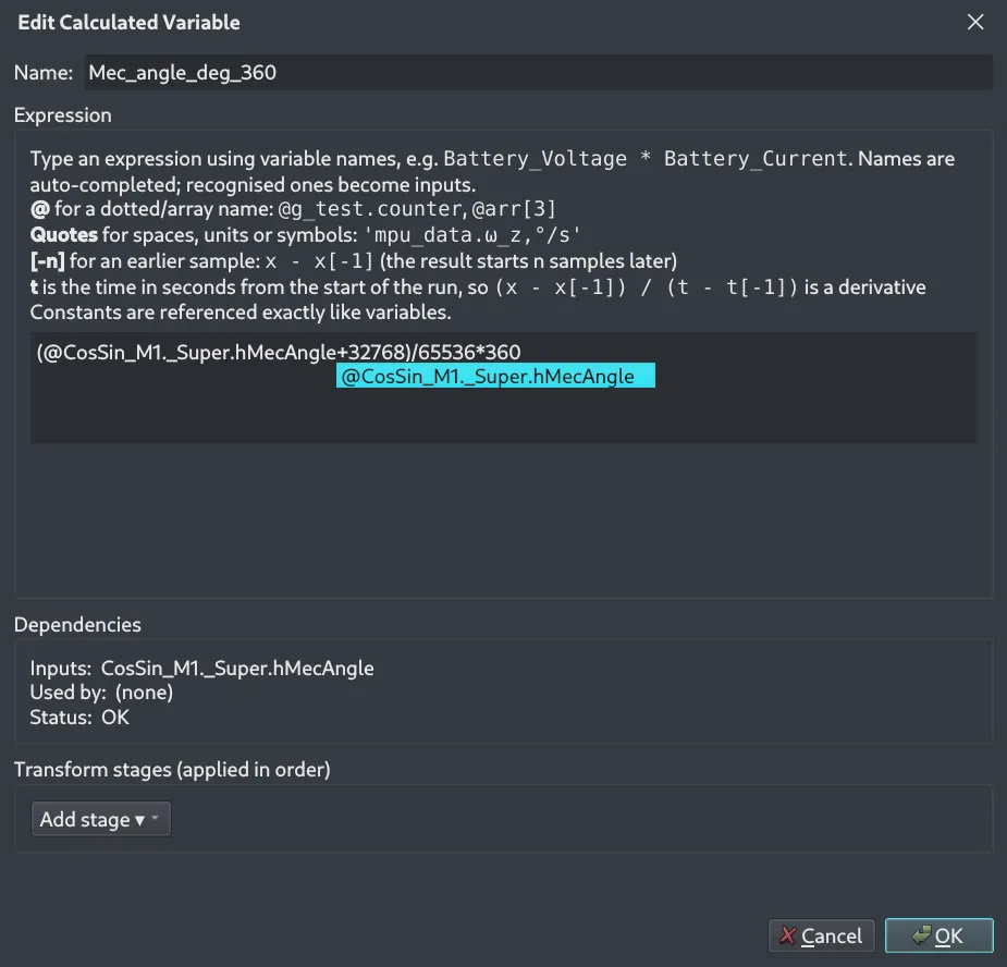
The Edit Calculated Variable dialog: a name, an expression with a variable name being auto-completed, a dependencies panel showing the inputs and status, and a list of transform stages

Compare Raw and Derived Signals

Plot a calculated channel next to the signal it was derived from.
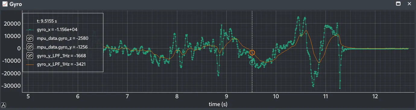
A time plot of a raw gyroscope axis with a calculated 1 Hz low-pass-filtered version of it drawn over the top

Ready to try it yourself?