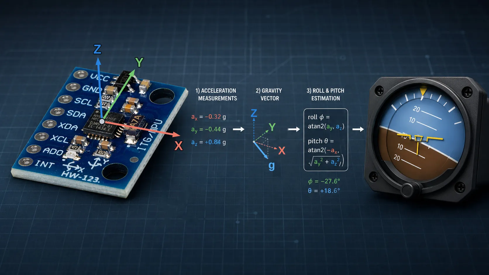
MPU6050 Roll and Pitch: Estimating Attitude from the Gravity Vector

In the previous experiments, we progressively turned the MPU6050 from an unknown sensor into a reasonably well-characterized measurement device.

We brought it up, calibrated the accelerometer and gyroscope, verified the sampling timing, and investigated the noise characteristics of the measurements.

In this experiment, we will take the next step: using the accelerometer measurements to estimate the orientation of the sensor.

The approach will be deliberately simple. We will treat the measured acceleration as a three-dimensional vector and transform it into a two-dimensional attitude vector:

$$\begin{bmatrix} a_x \\ a_y \\ a_z \end{bmatrix} \longrightarrow \begin{bmatrix} \mathrm{roll} \\ \mathrm{pitch} \end{bmatrix}$$

This gives us a compact attitude-estimation function that can later become one component of a more complete inertial-navigation or sensor-fusion system.

1. The Accelerometer Can Measure More Than Acceleration

An accelerometer measures specific force rather than directly measuring velocity or position.

When the sensor is stationary, the dominant component of this measurement is the Earth’s gravitational field. As a result, the accelerometer gives us a useful reference vector even when the sensor itself is not moving.

For a stationary sensor, we can therefore consider the measurement

$$\mathbf{a} = \begin{bmatrix} a_x \\ a_y \\ a_z \end{bmatrix}$$

to be an observation of the gravity vector expressed in the sensor’s coordinate system.

The important point is that gravity does not disappear when we rotate the sensor.

Instead, its components along the sensor’s X, Y, and Z axes change.

If the sensor is lying flat, most of the gravity vector appears along one axis. If we tilt the sensor, gravity is distributed between multiple axes.

The direction of this vector therefore contains information about the sensor’s orientation.

2. From Three Measurements to a Vector

The MPU6050 gives us three independent accelerometer measurements: $a_x$, $a_y$ and $a_z$.

We can combine them into a single vector:

$$\mathbf{a} = \begin{bmatrix} a_x \\ a_y \\ a_z \end{bmatrix}$$

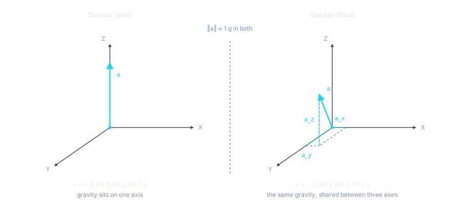Figure 1 — The three accelerometer channels are the components of one vector. Rotating the sensor moves gravity between the axes; the length of the vector does not change.

This is more useful than considering each accelerometer channel independently.

For a stationary sensor, the vector represents gravity in the sensor coordinate system.

Its magnitude should be approximately equal to gravitational acceleration:

$$\sqrt{a_x^2 + a_y^2 + a_z^2} \approx g$$

where $g$ is approximately 9.81 m/s².

This gives us an important sanity check.

When the sensor is rotated without being translated, the individual components should change, but the magnitude of the vector should remain approximately constant.

3. First Experiment: Rotate the Sensor

Before calculating any angles, let’s look at the accelerometer vector itself.

We place the MPU6050 in a known orientation and then slowly rotate it around one of its axes.

The three accelerometer channels are recorded using EmbedStudio.

The expected behavior is straightforward: as the sensor rotates, the gravity component moves from one sensor axis to another.

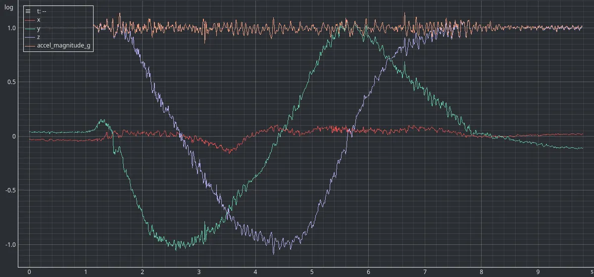Figure 2 — One rotation about the X axis. y and z trade the whole of gravity between them while x stays near zero, and accel_magnitude_g holds at 1 g — mean 1.000 g across the turn, so the vector is rotating rather than growing.

The individual signals change substantially, but they are not independent. Together, they describe the same gravity vector.

As the sensor rotates, the direction of this vector relative to the sensor coordinate system changes. This direction is what we will use to determine the sensor’s attitude.

The next step is therefore to convert the three-dimensional acceleration vector into a two-dimensional attitude representation.

4. Calculating Roll and Pitch from the Acceleration Vector

Once we have the calibrated acceleration vector, we can directly calculate the sensor’s tilt relative to gravity.

The two angles we are interested in are roll and pitch.

For the coordinate system used in this experiment, roll is calculated from the Y and Z components of the acceleration vector:

$$\mathrm{roll} = \operatorname{atan2}(a_y,\, a_z)$$

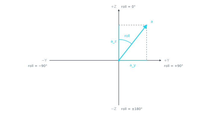Figure 3 — Roll is the direction of the gravity vector inside the YZ plane, measured from the Z axis. Because atan2 reads the signs of both components, it covers the whole circle — and the two ends of that circle, +180° and −180°, are the same orientation.

Pitch is calculated from the X component and the magnitude of the gravity projection onto the YZ plane:

$$\mathrm{pitch} = \operatorname{atan2}\left(-a_x,\; \sqrt{a_y^2 + a_z^2}\right)$$

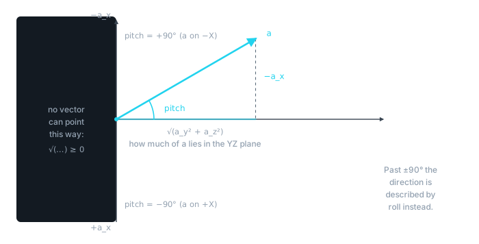Figure 4 — Pitch is the angle between the vector and its own shadow in the YZ plane. That shadow is a square root, so it only ever points one way — which is what confines pitch to −90°…+90°, and section 6.3 is that constraint showing up in real data.

The use of atan2() is important because it allows the calculation to account for the signs of the vector components and determine the correct quadrant.

The two equations use the same acceleration vector, but each extracts a different aspect of its direction.

There is an important limitation to this approach. The accelerometer can determine the direction of gravity, but gravity does not provide a reference for rotation around itself. Consequently, roll and pitch can be estimated from the accelerometer, but yaw cannot.

This also means that these equations describe the current orientation relative to gravity. They do not track how the sensor arrived at that orientation. As we will see later in the experiment, this distinction becomes particularly interesting when the sensor is rotated beyond 90°.

With the mathematical relationship established, we can now turn it into a small, reusable function that takes the acceleration vector as its input and returns the calculated roll and pitch.

5. Turning the Calculation into a Function

The mathematical calculation can now be isolated into a small, reusable function.

The function does not need to know anything about the MPU6050 itself. It only needs the calibrated acceleration vector

$$\mathbf{a} = \begin{bmatrix} a_x \\ a_y \\ a_z \end{bmatrix} \longrightarrow \begin{bmatrix} \mathrm{roll} \\ \mathrm{pitch} \end{bmatrix}$$

and produces the corresponding roll and pitch angles.

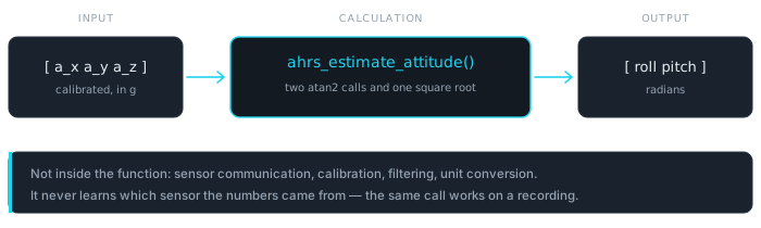Figure 5 — The whole abstraction. Three numbers in, two numbers out, and nothing about the sensor in between.

In C, we can represent the input and output using simple vector types:

enum {
    VECTOR_INDEX_X = 0,
    VECTOR_INDEX_Y = 1,
    VECTOR_INDEX_Z = 2,
    VECTOR_3F_N_ELEMENTS = 3,
};

typedef union {
    struct {
        float x;
        float y;
        float z;
    };
    float v[VECTOR_3F_N_ELEMENTS];
} vector_3f_t;

typedef struct {
    float roll;
    float pitch;
} ahrs_attitude_t;

The interface can then be kept simple:

void ahrs_estimate_attitude(const vector_3f_t* const acceleration,
        ahrs_attitude_t* const attitude);

The implementation directly follows the equations from the previous section:

void ahrs_estimate_attitude(const vector_3f_t* const acceleration,
        ahrs_attitude_t* const attitude)
{
    attitude->roll = atan2(acceleration->y, acceleration->z);
    attitude->pitch = atan2(-acceleration->x,
            sqrtf(acceleration->y * acceleration->y
                    + acceleration->z * acceleration->z));
}

There is deliberately no MPU6050-specific code in this function.

The function does not perform sensor communication, calibration, filtering, or unit conversion. Those operations belong to other parts of the system.

Its only responsibility is to transform a calibrated acceleration vector into a gravity-referenced roll and pitch estimate.

This separation makes the calculation easy to test independently and allows it to be reused with acceleration data coming from a different source, including previously recorded measurements.

The result is a very compact abstraction:

a  →  ahrs_estimate_attitude()  →  (roll, pitch)

The next step is to connect this function to the measured data and observe how the calculated angles behave during controlled rotations.

6. Understanding the Attitude Representation

With the calculation implemented, we can now connect it to the measured accelerometer data and investigate how the resulting roll and pitch behave during rotation.

This is where the choice of attitude representation becomes particularly interesting.

The accelerometer provides the direction of the gravity vector at each instant. It does not provide information about the history of the sensor’s rotation.

Our equations convert this gravity direction into two angles using a particular convention:

$$\mathrm{roll} \in [-180^\circ,\, 180^\circ] \qquad\text{and}\qquad \mathrm{pitch} \in [-90^\circ,\, 90^\circ]$$

Let’s see the consequences of this convention experimentally.

6.1 Rotation Around the Roll Axis

We start with the board approximately level and slowly rotate it around the X axis.

During this rotation, the gravity vector changes primarily in the YZ plane.

The calculated roll follows the physical rotation of the board, while pitch remains approximately constant.

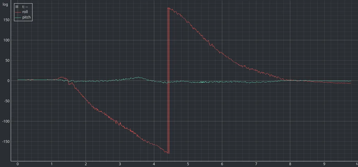Figure 6 — Roll (red) tracks the full turn; pitch (green) stays within 10° of zero. The vertical line at 4.4 s is the whole of the discontinuity: two consecutive samples read −179.1° and then +179.9°, a real movement of about a degree reported as a 359° jump.

As the board passes through 180°, the calculated roll changes from values close to +180° to values close to −180°.

For example, the output may contain a sequence such as 178°, 179°, −180°, −179°.

The apparent jump is not a physical discontinuity.

It is simply the boundary of the chosen angular representation. The orientations represented by +180° and −180° are identical.

This is a normal consequence of using atan2() to represent an angle within the range −180°…+180°.

6.2 Rotation Around the Pitch Axis

We now repeat the experiment by slowly rotating the board around the Y axis.

This time, the behavior is different.

We might intuitively expect the pitch angle to continuously follow the physical rotation, 0° → 90° → 180°.

Instead, the calculated pitch reaches approximately −90° and then starts moving back toward 0°.

At the same time, the calculated roll moves toward approximately +180° or −180°.

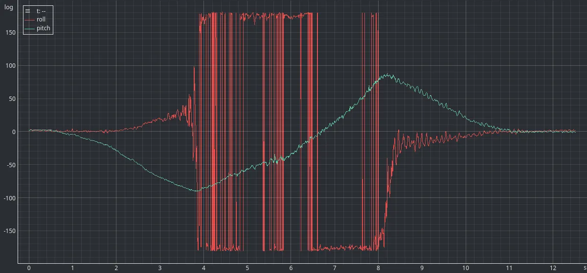Figure 7 — The board turns one way throughout. Pitch (green) reaches −89.7° near 3.9 s and then comes back, while roll (red) snaps to ±180° at exactly that moment and stays there until the board is the right way up again. The red band between 4 s and 8 s is roll sitting on the boundary of its own range, crossing between +180° and −180° on the noise.

This behavior is a direct consequence of how the two angles are defined.

6.3 Why Does Pitch Return After 90°?

Consider the acceleration vector $\mathbf{a} = [\,a_x\;a_y\;a_z\,]$. The pitch calculation is:

$$\mathrm{pitch} = \operatorname{atan2}\left(-a_x,\; \sqrt{a_y^2 + a_z^2}\right)$$

The square-root term is always non-negative:

$$\sqrt{a_y^2 + a_z^2} \geq 0$$

Consequently, the resulting pitch is restricted to:

$$-90^\circ \leq \mathrm{pitch} \leq +90^\circ$$

When the board is rotated beyond 90°, the gravity vector can no longer be represented by increasing pitch while maintaining this constraint.

Instead, the orientation is represented using the other angle.

The board that we might describe physically as having a pitch of 135° can be represented by the gravity-based attitude calculation as an orientation with approximately roll = 180° and pitch = 45°.

Both representations correspond to the same direction of gravity.

This is an important distinction.

The accelerometer-based calculation does not measure how far the board has rotated from some starting position. It determines the current direction of gravity and expresses that direction using our chosen roll/pitch convention.

Therefore, when the board is turned upside down, the calculation does not need to report a pitch angle greater than 90°. The same gravity direction can be represented by changing the roll angle instead.

This also explains the behavior observed during the experiment: as pitch approaches 90°, the attitude representation transitions toward a roll of approximately 180°.

The result is not an error in the calculation. It is a consequence of representing a three-dimensional orientation using this particular pair of angles.

It also highlights an important limitation of accelerometer-only attitude estimation: the accelerometer provides the direction of gravity, but not the rotational history of the sensor.

For our purposes, this representation is perfectly suitable for measuring tilt relative to gravity. If we later want to track continuous rotations through arbitrary orientations, we will need to incorporate information from the gyroscope.

7. How Stable Is the Estimated Attitude?

So far we have focused on the geometric behavior of the attitude estimator. We have seen how the direction of the gravity vector can be transformed into roll and pitch, and how the chosen representation behaves during large rotations.

The next question is how stable the calculated attitude is when the sensor is stationary.

Even when the MPU6050 is not moving, the accelerometer measurements contain noise. Since roll and pitch are calculated directly from these measurements, this noise propagates into the resulting attitude estimate.

To investigate this effect, we placed the sensor on a stable surface and recorded the calculated roll and pitch using two different MPU6050 Digital Low-Pass Filter (DLPF) configurations:

• DLPF configured to 260 Hz;
• DLPF configured to 22 Hz.

These are the same configurations investigated in Experiment #005, where we characterized their effect on accelerometer noise.

The recorded attitude signals were analyzed using the Analysis instrument in EmbedStudio.

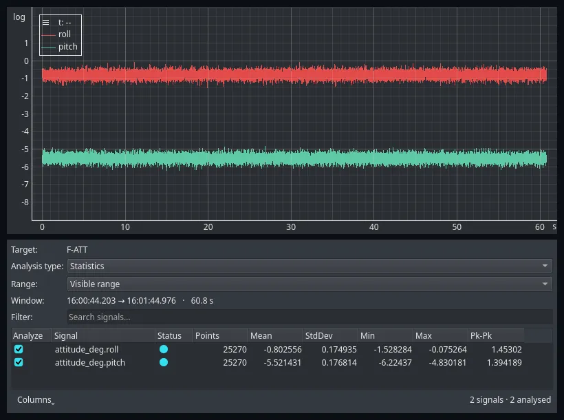Figure 8 — One stationary minute at DLPF 260 Hz, measured by the Analysis panel over the whole recording. Roll sits at −0.803° ± 0.175°, pitch at −5.521° ± 0.177°; the two bands are the noise this configuration leaves in the angle.

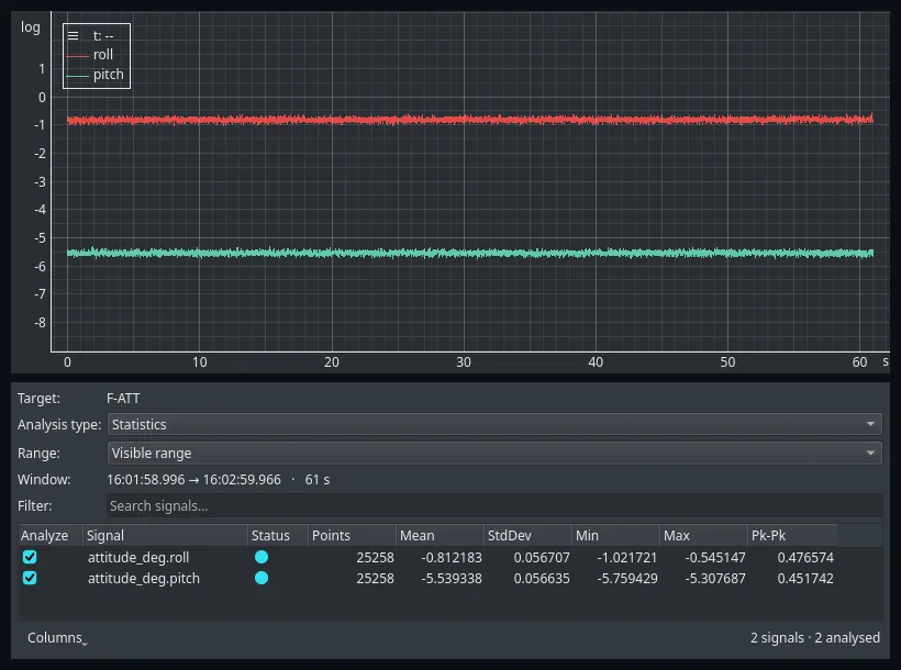Figure 9 — The same minute, the same y axis, the DLPF at 22 Hz. Both bands are about a third as deep, and the means barely moved — −0.812° and −5.539° against −0.803° and −5.521°. Filtering changed the spread, not the answer.

The resulting statistics are summarized below:

Configuration	Roll σ	Roll pk-pk	Pitch σ	Pitch pk-pk
DLPF 260 Hz	0.175°	1.453°	0.177°	1.394°
DLPF 22 Hz	0.057°	0.477°	0.057°	0.452°

The standard deviation provides a useful measure of the short-term noise of the attitude estimate, while the peak-to-peak value shows the total observed variation during the measurement interval.

The results show that reducing the DLPF bandwidth from 260 Hz to 22 Hz reduces the variation of the calculated roll and pitch. Both angles improved by a factor of about three, and so did the acceleration channels they are calculated from: the standard deviation of X and Y fell from 3.1 mg to 1.0 mg, and Z from 4.7 mg to 1.5 mg.

This is a direct consequence of the relationship between the accelerometer measurements and the attitude calculation. The attitude estimator operates directly on the acceleration vector, so noise in the individual acceleration channels propagates into the calculated angles.

The experiment therefore demonstrates a complete chain from sensor noise to a higher-level measurement:

Accelerometer noise
        ↓
Acceleration vector
        ↓
Roll / pitch calculation
        ↓
Attitude noise

This also provides a direct connection to the results from Experiment #005. The reduction in acceleration noise observed there produces a corresponding improvement in the stability of the calculated attitude.

However, reducing the DLPF bandwidth comes with the same trade-off discussed in Experiment #005. A lower bandwidth reduces noise but increases signal delay and limits the response to rapid changes.

For applications where the attitude changes slowly, the reduced noise may be more important than the additional delay. For highly dynamic motion, a higher bandwidth may provide a better compromise between noise and responsiveness.

8. What Happens When the Sensor Moves?

So far, the sensor has been either stationary or rotated slowly enough that gravity remains the dominant component of the accelerometer measurement.

But what happens when the sensor experiences actual linear acceleration?

The accelerometer does not measure gravity separately from other acceleration. It measures their combined effect:

$$\mathbf{a}_\mathrm{measured} = \mathbf{g} + \mathbf{a}_\mathrm{motion}$$

where $\mathbf{g}$ is the gravity component and $\mathbf{a}_\mathrm{motion}$ is acceleration caused by the movement of the sensor.

Our attitude calculation assumes that the measured acceleration vector represents gravity. If the sensor is accelerating, this assumption is no longer valid.

For example, imagine holding the sensor level and accelerating it horizontally. The physical orientation of the sensor has not changed, but the measured acceleration vector now contains a horizontal component.

The attitude estimator interprets this additional acceleration as a change in the direction of gravity and therefore produces a change in the calculated roll or pitch.

Dynamic Experiment

To demonstrate this effect, we keep the sensor approximately at the same orientation while moving it back and forth.

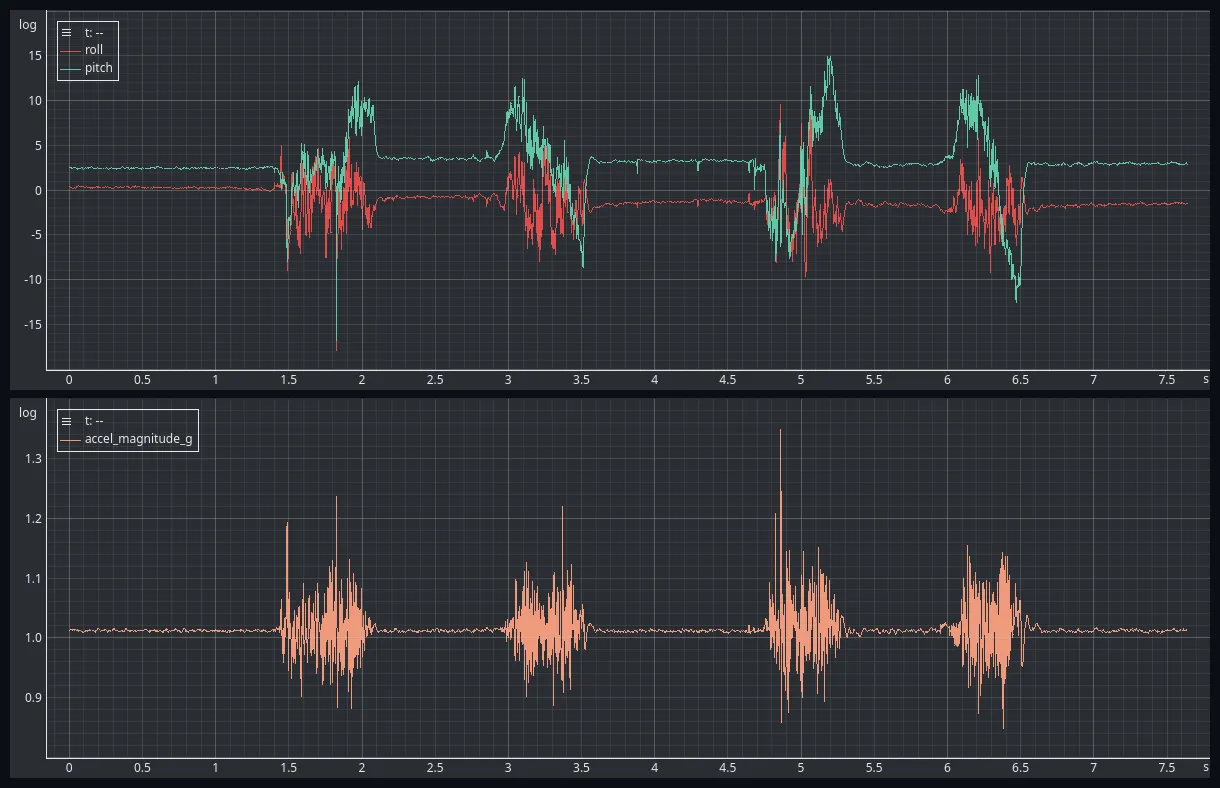Figure 10 — Four bursts of horizontal movement, with the board’s orientation unchanged throughout. Roll and pitch (top) swing by up to 18° and 19° away from their resting values, which held to better than 0.11° between the bursts. The magnitude (bottom) is the tell: 1.012 g while still, 0.85 g to 1.35 g while moving.

The calculated attitude changes during the movement even though the sensor’s physical orientation remains approximately unchanged.

This is not a failure of the atan2() calculation. The calculation is operating correctly on the information provided by the accelerometer. The problem is that the acceleration vector no longer represents gravity alone.

This experiment demonstrates a fundamental limitation of accelerometer-only attitude estimation:

An accelerometer can provide a reliable reference for tilt when gravity is the dominant acceleration, but it cannot distinguish gravity from acceleration caused by motion.

Filtering can reduce some of the resulting disturbance, but it cannot solve the underlying problem. A filter cannot determine whether a change in the measured acceleration is caused by rotation, gravity, or linear motion.

This is where the gyroscope becomes important. The gyroscope provides information about angular velocity and is not affected by linear acceleration in the same way as the accelerometer.

Combining the two measurements allows us to use the strengths of both sensors: the accelerometer provides a long-term reference to gravity, while the gyroscope provides continuous information about rotational motion.

This is the fundamental motivation for sensor fusion.

9. What Have We Learned?

In this experiment, we moved from calibrated accelerometer measurements to a practical estimate of the sensor’s attitude.

Starting with the three calibrated acceleration channels, we treated them as a three-dimensional vector representing the direction of gravity. From this vector, we calculated roll and pitch using a simple pair of atan2()-based equations.

The experiments demonstrated several important properties of this approach.

First, the calculation is remarkably simple. No integration or complex estimation algorithm is required to obtain a useful tilt estimate from the accelerometer.

Second, the chosen roll and pitch representation has important consequences. Roll can span the full −180° to +180° range, while pitch is limited to −90° to +90°. When the sensor is rotated beyond 90° pitch, the orientation is represented by a change in roll instead. This is a property of the angle representation, not an error in the calculation.

Third, the quality of the attitude estimate is directly affected by accelerometer noise. The comparison of the 260 Hz and 22 Hz DLPF configurations demonstrated how reducing measurement noise produces a more stable attitude estimate.

Finally, we observed the fundamental limitation of accelerometer-only attitude estimation. When the sensor experiences significant linear acceleration, the measured acceleration vector no longer represents gravity alone, and the calculated attitude can therefore deviate from the actual orientation.

The accelerometer is consequently a very useful source of absolute tilt information, but it is not sufficient for reliable attitude tracking during arbitrary motion.

This leads naturally to the gyroscope: tracking rotational motion with it and combining it with the accelerometer to obtain a more robust attitude estimate.

Experiment data

The raw datasets used in this experiment are publicly available in the EmbedStudio Experiments repository.

The dataset contains:

• a short stationary capture;
• the rotation about the X axis used in section 6.1;
• the rotation about the Y axis used in section 6.2;
• the two stationary one-minute captures at DLPF 260 Hz and 22 Hz used in section 7;
• the linear-movement capture used in section 8.

All datasets are provided as HDF5 files and can be downloaded and opened with EmbedStudio or another compatible HDF5 tool.

References

• InvenSense, MPU-6000 and MPU-6050 Register Map and Descriptions, Rev. 4.2 (RM-MPU-6000A-00, 2013) — PDF. Source of the DLPF_CFG bandwidth table behind the two configurations compared in section 7.

Next Experiment

Experiment #007: When Accelerometer Roll Estimation Fails

Section 6 showed the roll angle swinging towards 180° as pitch approached 90°, and section 7 measured how steady that angle is while the sensor sits level. Those two results meet at an uncomfortable question: what is the roll estimate worth near vertical?

The next experiment answers it. As gravity swings onto the X axis, the YZ projection that the roll equation depends on shrinks into the noise floor, and the estimate starts moving through hundreds of degrees while the board is stationary. That failure is measured, then a regularization term is added to the denominator to suppress it — five coefficients computed side by side on-target — and the systematic error the same term introduces at ordinary angles is measured against it.