MPU6050 Noise and Filtering: How Much Is Noise, and What Does a Filter Cost?

In the previous MPU6050 experiments, the sensor was operated with its built-in low-pass filter enabled. This works well for normal operation, but it leaves an important question unanswered:

How much of the variation we see in the sensor output is actually noise, and how does filtering affect it?

In this experiment, we step back and characterize the sensor noise before applying filtering.

We start with the MPU6050 configured for its widest bandwidth and acquire stationary accelerometer and gyroscope data at 1 kSPS. The data is then analyzed both in the time domain and frequency domain using EmbedStudio’s FFT and Spectrogram instruments.

After establishing the baseline, we repeat the experiment with the MPU6050’s internal DLPF configured for approximately 44 Hz and 20 Hz.

Finally, instead of relying exclusively on the sensor’s hardware filter, we apply software low-pass filters to the same raw dataset. Three cutoff frequencies — 22 Hz, 10 Hz, and 5 Hz — are tested.

The final experiment investigates the price paid for additional filtering: response delay.

Experimental setup

The experiment uses the same STM32-based MPU6050 setup developed in the previous experiments.

The sensor is configured as follows:

Parameter	Configuration
Accelerometer range	±2 g
Gyroscope range	±250 °/s
Acquisition rate	1 kSPS
Sensor	MPU6050

For the initial measurement, the MPU6050 is configured for its widest available bandwidth.

Three hardware configurations are investigated:

Configuration	DLPF_CFG	SMPLRT_DIV	DLPF bandwidth	Purpose
A	0	7	~260 Hz	Maximum-bandwidth baseline
B	3	0	~44 Hz	Hardware filtering
C	4	0	~20 Hz	Hardware filtering

The divider changes with the bandwidth because DLPF_CFG = 0 puts the gyroscope output rate at 8 kHz, while every other setting puts it at 1 kHz. All three configurations therefore run at 1 kSPS.

The sensor remains stationary during all three noise measurements.

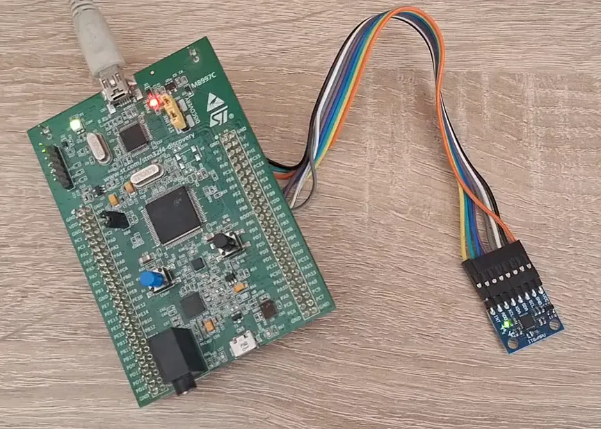Figure 1 — Experimental setup used for the noise and filtering measurements.

The firmware used for these measurements is tagged experiment_005. The bandwidth is a single #define there: MPU6050_DLPF_BANDWIDTH selects the setting, and the divider is derived from it, so the two cannot disagree.

The raw measurements are available as HDF5 datasets in the EmbedStudio Experiments repository.

Establishing the noise baseline

The first capture uses the maximum-bandwidth configuration.

With the sensor sitting completely still, the output is not constant. Both the accelerometer and gyroscope show continuous variations around their mean values.

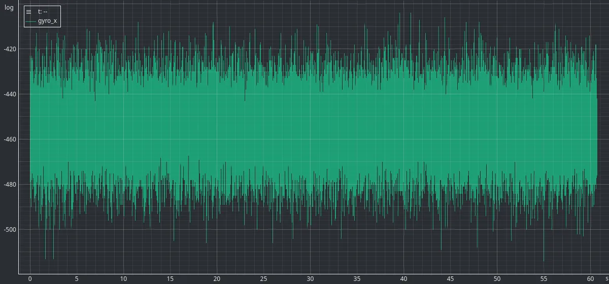Figure 2 — Stationary gyroscope output with the MPU6050 configured for maximum bandwidth.

The time-domain signal tells us how large the variations are, but it does not tell us where they come from.

For that, we need to look at the signal in the frequency domain.

Looking at the noise with FFT

EmbedStudio’s FFT instrument provides a convenient way to examine the frequency content of the stationary sensor output.

The maximum-bandwidth capture does not show any clearly dominant narrow-band peaks. Instead, the noise is distributed over a broad frequency range.

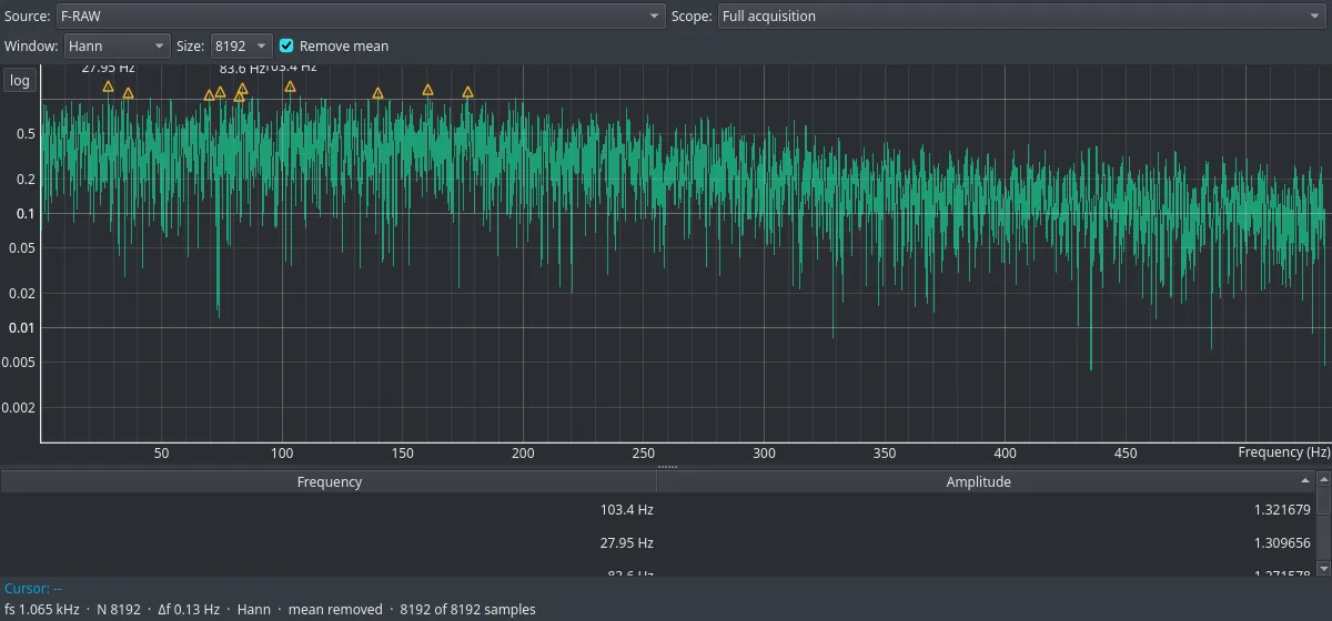Figure 3 — FFT of the stationary MPU6050 output at maximum bandwidth.

For the gyroscope channels, the noise floor remains approximately flat up to roughly 240–250 Hz before falling toward the Nyquist frequency.

The accelerometer channels show a similar behavior, with the transition occurring in the same region, approximately between 235 and 250 Hz depending on the axis.

This is exactly the kind of signal for which a low-pass filter can be useful: there is significant high-frequency energy that may not be relevant to the application.

But before filtering the signal, it is useful to determine whether this behavior remains stable over time.

Looking at the noise with a spectrogram

The FFT gives us the frequency content averaged over the acquisition interval. A spectrogram adds another dimension by showing how that spectrum changes with time.

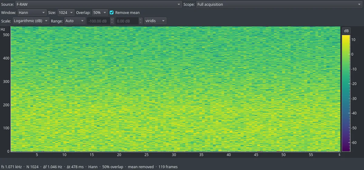Figure 4 — Spectrogram of the stationary MPU6050 output at maximum bandwidth.

The spectrum remains stable throughout the entire recording.

There are no obvious intermittent disturbances or time-varying frequency components.

This is useful confirmation that the observed noise is not caused by a short-lived event in the experiment. The spectral characteristics are stable during the measurement.

What happens when we enable the internal DLPF?

Now we repeat the measurement with the MPU6050’s internal DLPF configured for approximately 44 Hz.

The difference is immediately visible in the FFT.

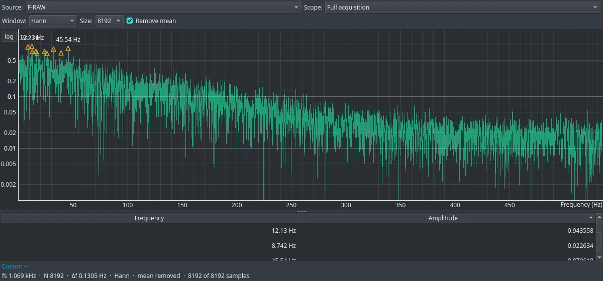Figure 5 — FFT with the MPU6050 internal DLPF configured for approximately 44 Hz.

The spectrum is approximately flat only through the tens-of-hertz range. Above that region, the noise is progressively attenuated.

Depending on the sensor channel, the transition occurs at approximately 42–46 Hz.

At 500 Hz, the measured spectrum is approximately 27–29 dB lower than the low-frequency noise floor.

Reducing the bandwidth further produces an even stronger effect.

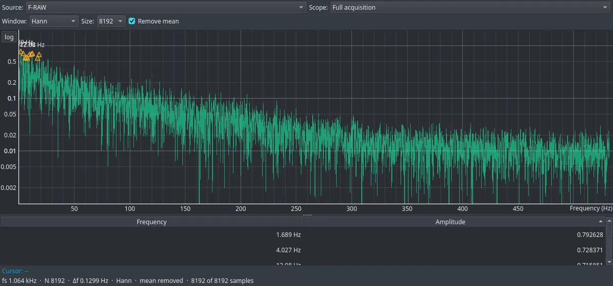Figure 6 — FFT with the MPU6050 internal DLPF configured for approximately 20 Hz.

The transition now occurs at approximately 21–25 Hz depending on the channel, with attenuation reaching approximately 30–34 dB at 500 Hz.

All three FFT captures were inspected using the same frequency and amplitude scales, making the effect of changing the DLPF configuration directly comparable.

Quantifying the noise reduction

The FFT clearly shows that high-frequency content is being removed, but we can also quantify the effect using the time-domain data.

For a stationary sensor, standard deviation is a useful measure of the noise amplitude.

The mean value represents the sensor’s static output — for example, the gyroscope bias or the accelerometer’s response to gravity — while the standard deviation describes the variations around that mean.

Standard deviation of the stationary sensor output

Channel	260 Hz — StdDev	44 Hz — StdDev	20 Hz — StdDev	Reduction 260 → 20 Hz
Gyro X	12.944	5.478	3.983	69.2 %
Gyro Y	12.012	5.231	3.819	68.2 %
Gyro Z	10.472	4.593	3.262	68.8 %
Accel X	50.898	22.993	16.337	67.9 %
Accel Y	50.765	23.043	16.521	67.5 %
Accel Z	75.477	34.529	24.358	67.8 %

Table 1 — Standard deviation of the stationary MPU6050 outputs at three internal DLPF settings. Values are expressed in LSB.

The result is remarkably consistent.

Moving from the maximum-bandwidth configuration to the approximately 20 Hz configuration reduces the standard deviation by approximately 67–69 % on every measured axis.

So the frequency-domain observation has a clear time-domain counterpart: reducing the sensor bandwidth substantially reduces the measured noise.

Why not use RMS?

At first glance, RMS might seem like an obvious metric for comparing the signals.

However, the sensor outputs contain substantial DC components.

For example, the Gyro X signal has a mean of approximately −455 LSB, while its noise standard deviation is only approximately 13 LSB.

The RMS value is therefore dominated by the sensor’s mean value:

RMS² ≈ μ² + σ²

Filtering reduces σ, but it does not significantly change μ.

As a result, the RMS values of the filtered signals remain almost identical even though their noise is substantially lower.

For this experiment, standard deviation is therefore the more useful metric for comparing noise levels.

Can we do the filtering in software?

The internal DLPF is convenient, but it is not the only option.

To investigate software filtering, we take the original maximum-bandwidth capture and process it offline.

This is particularly useful experimentally because every software filter operates on exactly the same raw data.

We test three cutoff frequencies:

• 22 Hz
• 10 Hz
• 5 Hz

This lets us compare different filter settings without introducing variation between separate physical measurements.

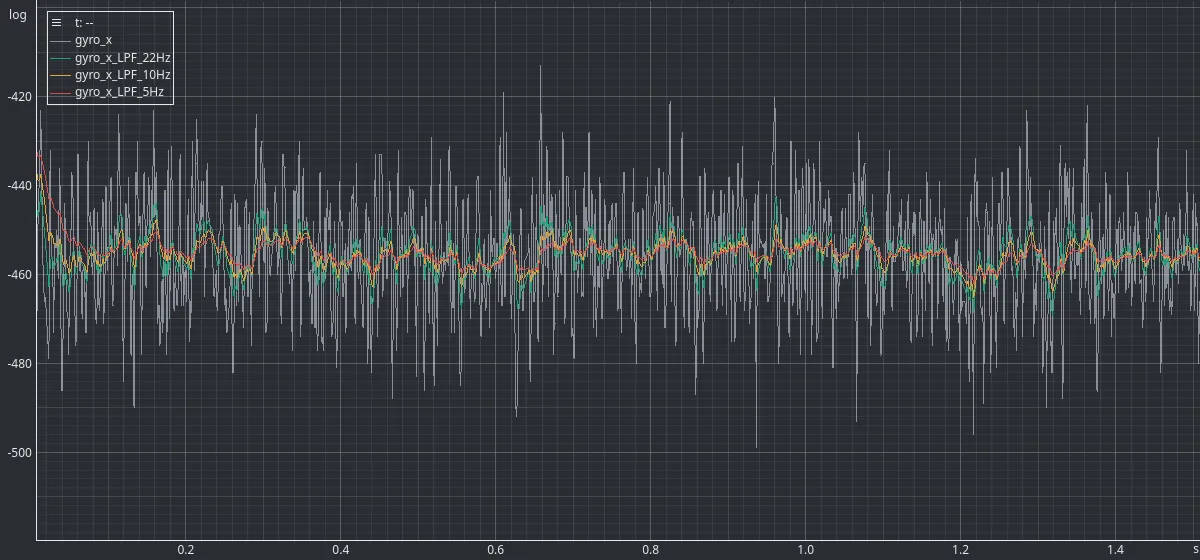Figure 7 — Effect of software low-pass filtering on the stationary gyroscope signal.

The noise reduction is substantial even with the 22 Hz filter.

Standard deviation after software filtering

Channel	Raw — StdDev	22 Hz — StdDev	10 Hz — StdDev	5 Hz — StdDev
Gyro X	12.944	4.240	2.940	2.132
Gyro Y	12.012	3.929	2.713	1.953
Gyro Z	10.472	3.406	2.339	1.657
Accel X	50.898	17.039	11.858	8.523
Accel Y	50.765	16.979	11.786	8.426
Accel Z	75.477	25.287	17.659	12.680

Table 2 — Standard deviation of the raw and software-filtered sensor outputs. Values are expressed in LSB.

For Gyro X, for example, the standard deviation decreases from 12.944 to 4.240 with the 22 Hz filter — a reduction of approximately 67 %.

The 10 Hz and 5 Hz filters provide progressively stronger noise reduction.

This demonstrates that software filtering can be very effective.

But there is a catch.

The cost of filtering: response delay

A low-pass filter cannot reduce high-frequency noise without also affecting the response to high-frequency changes in the actual signal.

To evaluate this effect, a simple dynamic experiment was performed.

The sensor was repeatedly flipped around the Gyro X axis while observing both the raw signal and several software-filtered versions of the same signal.

The experiment used three filter configurations:

• 22 Hz LPF
• 10 Hz LPF
• 5 Hz LPF

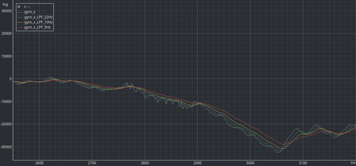Figure 8 — Gyro X response during a rotation experiment with software filtering.

All three filters successfully track the rotational motion.

However, the filtered signals increasingly lag behind the raw measurement as the cutoff frequency is reduced.

The effect is easy to observe when comparing the moments at which the signals begin to respond to the rotation.

The observed delays were approximately:

Filter	Gyro X StdDev	Noise Reduction	Observed Delay
Raw	12.944	—	—
22 Hz	4.240	67.2 %	~8 ms
10 Hz	2.940	77.3 %	~17 ms
5 Hz	2.132	83.5 %	~34 ms

Table 3 — Noise reduction and observed dynamic response for the Gyro X signal.

The relationship is clear.

Reducing the cutoff frequency improves noise suppression, but it also increases latency.

Interestingly, the first reduction in bandwidth provides the largest improvement.

Moving from the raw signal to the 22 Hz filter reduces the noise standard deviation by approximately 67 %.

Further reductions continue to suppress noise, but the improvement becomes progressively smaller while the delay continues to increase.

These delay values are measurements from this particular experiment and should not be interpreted as universal delay values for every implementation of a 22 Hz, 10 Hz, or 5 Hz filter.

The important observation is the trade-off:

Lowering the cutoff frequency reduces more noise, but increases the delay between a change in the real signal and the corresponding change in the filtered output.

For a slowly changing signal, 34 ms may be completely acceptable.

For a fast control loop, it may not.

Filtering cannot distinguish noise from useful motion

The FFT results also reveal an important limitation of low-pass filtering.

The filter knows nothing about whether a particular frequency component is “noise” or “useful signal.”

If both occupy the same frequency range, they are treated identically.

For example, suppose an application needs to measure motion containing useful components up to 15 Hz.

A 5 Hz low-pass filter may reduce the noise very effectively — but it will also remove part of the actual motion.

This means that simply choosing the lowest possible cutoff frequency is not a good strategy.

The correct cutoff frequency depends on the bandwidth of the signal we actually want to preserve.

Hardware or software filtering?

The experiment shows that both approaches are useful, but they serve somewhat different purposes.

The MPU6050’s internal DLPF is useful when we already know approximately what bandwidth the application requires.

It reduces the amount of high-frequency noise before the data reaches the MCU and therefore reduces the amount of unwanted information that needs to be processed.

Software filtering provides additional flexibility.

We can experiment with different cutoff frequencies without changing the sensor configuration, and we can potentially use more sophisticated filtering algorithms if the application requires them.

There is also an important practical benefit to acquiring the sensor at a relatively high rate and filtering in software: the raw information is still available.

During development, this makes it possible to experiment with different filters without repeating the physical measurement.

That is exactly what we did here — the 22 Hz, 10 Hz and 5 Hz filters were all applied to the same maximum-bandwidth capture.

Conclusion

This experiment started by removing as much filtering as practical from the MPU6050 signal path to establish a noise baseline.

FFT analysis showed that the stationary sensor output contains a broad noise spectrum extending well into the hundreds of hertz. Spectrogram analysis showed that this spectrum remains stable throughout the acquisition.

Activating the MPU6050’s internal DLPF significantly attenuated the high-frequency noise.

Moving from the maximum-bandwidth configuration to approximately 20 Hz reduced the standard deviation by approximately 67–69 % across all six accelerometer and gyroscope channels.

Software filtering produced a similar result.

A 22 Hz software low-pass filter reduced the Gyro X noise standard deviation by approximately 67 % while introducing only about 8 ms of observed delay.

Reducing the cutoff frequency further improved noise suppression:

• 10 Hz LPF: approximately 77 % noise reduction, approximately 17 ms delay
• 5 Hz LPF: approximately 84 % noise reduction, approximately 34 ms delay

The main lesson is therefore not simply that filtering reduces noise.

The first reduction in bandwidth removes a large portion of the high-frequency noise with relatively little impact on responsiveness.

Further reductions continue to suppress noise, but the improvements become progressively smaller while the response delay continues to increase.

For an embedded system, the correct filter is the one that provides sufficient noise suppression while preserving the bandwidth and response time required by the application.

Having access to the raw data makes this process significantly easier. Instead of guessing which filter configuration might be appropriate, we can capture the signal once, analyze its frequency content, and evaluate different filtering strategies before committing a configuration to firmware.

Experiment data

The raw datasets used in this experiment are publicly available in the EmbedStudio Experiments repository.

The dataset contains:

• the maximum-bandwidth stationary capture used as the noise baseline;
• the approximately 44 Hz and 20 Hz hardware-DLPF captures;
• the Gyro X rotation capture used to evaluate dynamic response.

The software-filtered 22 Hz, 10 Hz and 5 Hz results were derived from the maximum-bandwidth capture.

All datasets are provided as HDF5 files and can be downloaded and opened with EmbedStudio or another compatible HDF5 tool.

References

• InvenSense, MPU-6000 and MPU-6050 Register Map and Descriptions, Rev. 4.2 (RM-MPU-6000A-00, 2013) — PDF. Source of the DLPF_CFG bandwidth and delay table, and of the rule that DLPF_CFG = 0 puts the gyroscope output rate at 8 kHz.

Next Experiment

Experiment #006: The Accelerometer as an Inclination Sensor

The noise is characterised now, and so is the cost of removing it. The next question is what the accelerometer is good for once it is calibrated and filtered: measuring which way is down.

That turns a three-axis acceleration reading into an angle, and it brings a new set of problems with it. Gravity is only one of the accelerations the sensor feels, the geometry stops being linear away from level, and the noise measured here turns into an angle error whose size depends on the tilt.