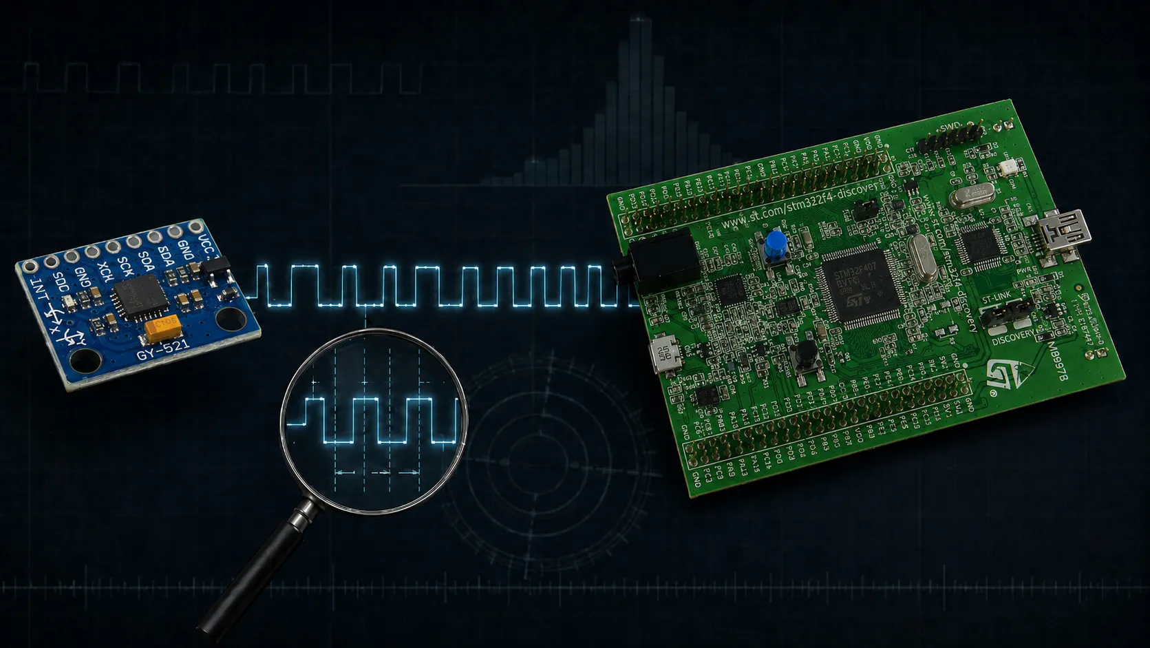
MPU6050 Timing and Sampling: Why a 1 kHz Sensor Does Not Sample Every 1000 µs

The bring-up article has one line in it that the rest of this series has been quietly standing on. While clearing the sleep bit, it says, it is worth selecting a gyroscope PLL as the sensor’s clock source instead of the internal oscillator.

That line came out of a measurement, and the measurement deserves more than a line. On its default clock source, this MPU6050 was 1.2 % away from the sample rate it had been configured for, and its sampling was ten times less steady. Nothing in the sensor data showed either. Every angle integrated from that data would have carried the error, and no amount of calibrating the gyroscope would have removed it.

That is what this article is about.

How close is 1 kHz to the real thing?

The MPU6050 can be configured for a nominal 1 kHz sample rate, and that sounds simple enough: one sample every millisecond.

But a real embedded system is not an ideal clock. The sensor has its own timing system, the MCU has its own clock reference, and firmware execution adds effects of its own. The sample rate register does not really set a period. It sets a divider, and the period it divides is whatever the sensor’s clock happens to be running at.

For many applications, small timing variations are irrelevant. For others, they matter a great deal. Gyroscope integration depends directly on the elapsed time between measurements. Frequency analysis depends on the sampling frequency. Sensor-fusion algorithms need to know how much time has passed between updates.

So instead of assuming that 1 kHz means exactly 1000 µs, let’s measure it.

The Experiment

The sensor’s DATA_RDY signal is connected to an STM32 GPIO configured to generate an interrupt. Every time the MPU6050 indicates that a new sample is available, the interrupt handler captures the current value of the DWT cycle counter.

For consecutive samples, the firmware calculates:

dt[n] = t[n] - t[n-1]

The measured dt is then recorded alongside the sensor data.

The important point is that the timing is measured inside the MCU, a few cycles from the event being investigated. We are not measuring the time between packets arriving at a PC. That would include communication and software delays which have nothing to do with the sensor’s actual sampling timing.

Why Not Use the Standard HAL Tick?

The STM32 HAL already provides convenient timing functions, so why introduce a separate timing module?

The answer is resolution.

A typical HAL system tick provides a time base with millisecond resolution. That is perfectly adequate for timeouts, delays and task scheduling, but it is not suitable for investigating variation around a 1 ms sampling period. Consider these intervals:

998 µs    1001 µs    1003 µs    997 µs

They are all the same number of milliseconds. A ruler graduated in millimetres cannot measure the difference between two objects a millimetre long.

The DWT cycle counter works at the MCU core-clock resolution instead. It is a free-running 32-bit register inside the Cortex-M core that increments once per core clock cycle, so at 168 MHz it resolves 5.95 ns. Reading it is a single load from a memory-mapped address — no peripheral, no interrupt and no HAL call in the path, which is what makes it usable from inside a handler.

Two properties are worth knowing before relying on it. It rolls over every 2³² cycles, which at 168 MHz is 25.6 s. That does not matter for intervals, because unsigned subtraction in C is defined modulo 2³², so the difference of two timestamps stays exact as long as the interval itself is shorter than the wraparound period. One millisecond has a comfortable margin. And on some parts the DWT is held in reset until a debugger attaches, so the counter has to be enabled explicitly rather than assumed.

This makes the DWT particularly useful for:

• measuring short time intervals;
• measuring firmware execution time;
• investigating interrupt latency;
• evaluating sampling jitter.

The timing functionality used in this experiment is implemented as a reusable project module. Its detailed implementation and API are outside the scope of this article and will be covered separately.

Measuring the Sampling Interval

The timing reference is the MPU6050 DATA_RDY event. Each event indicates that a new sensor sample is available. The STM32 captures the current DWT counter value and compares it with the previous one, and the difference between the two is the actual interval between consecutive sensor events.

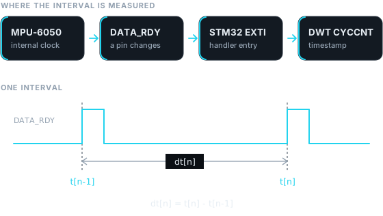Figure 1 — Measuring the sampling interval. Two consecutive MPU6050 DATA_RDY events are timestamped by the STM32, and the difference between the timestamps gives the measured dt.

This gives us something the MPU6050 configuration registers cannot provide: an actual measurement of the timing produced by the sensor. SMPLRT_DIV says what the sensor was asked to do. The interval between two data-ready edges says what it did.

Experimental Setup

The hardware is the same basic platform used in the previous MPU6050 experiments:

• STM32F4 Discovery
• GY-521 module containing the MPU6050
• I²C connection
• MPU6050 DATA_RDY signal connected to the STM32

The sensor is configured for a nominal 1 kHz output rate with the digital low-pass filter enabled.

The STM32 is clocked from the external HSE oscillator rather than the internal HSI. This provides a more stable and predictable clock reference for the DWT-based timing measurement, and a timing reference is exactly the wrong place to save a crystal. Every number below is quoted against the resulting 168 MHz core clock.

The I²C interface is used to read the sensor data, but it is not the timing reference for this experiment.

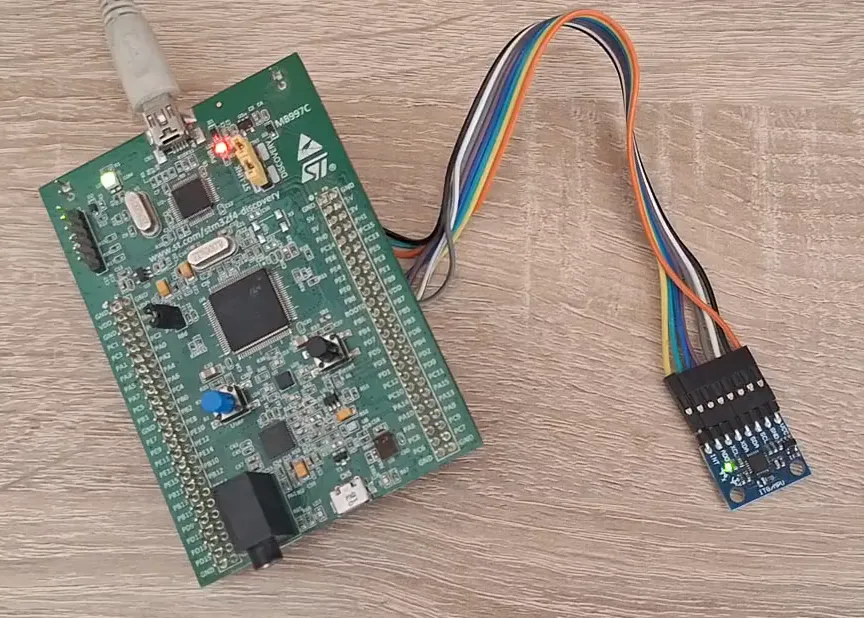Figure 2 — Experimental setup showing the STM32F4 Discovery and GY-521/MPU6050, with the I²C connection and the DATA_RDY signal used as the timing reference.

The distinction is important. The I²C transaction tells the MCU how to obtain the data. The DATA_RDY event tells us when the sensor indicates that a new sample is available. For this experiment, the second one is the timing reference, so a slow or retried I²C transaction cannot move the result.

Part 1 — What Is the Real Sampling Period?

The First Measurement

The nominal sampling period for 1 kHz is:

Fs = 1000 Hz
T  = 1 / Fs = 1 ms = 1000 µs

So the first expectation is simple: dt ≈ 1000 µs.

But the first measurement did not look as clean as expected. Instead of a tight distribution around 1000 µs, the measured intervals showed a substantial deviation from the nominal value. Averaged over 41,729 samples, the observed period was 987.7 µs, which corresponds to an effective sampling frequency of:

Fs = 1 / 987.7 µs = 1012.4 Hz

This was unexpected. The MPU6050 was configured for 1 kHz, so why were the measured intervals so far from 1 ms?

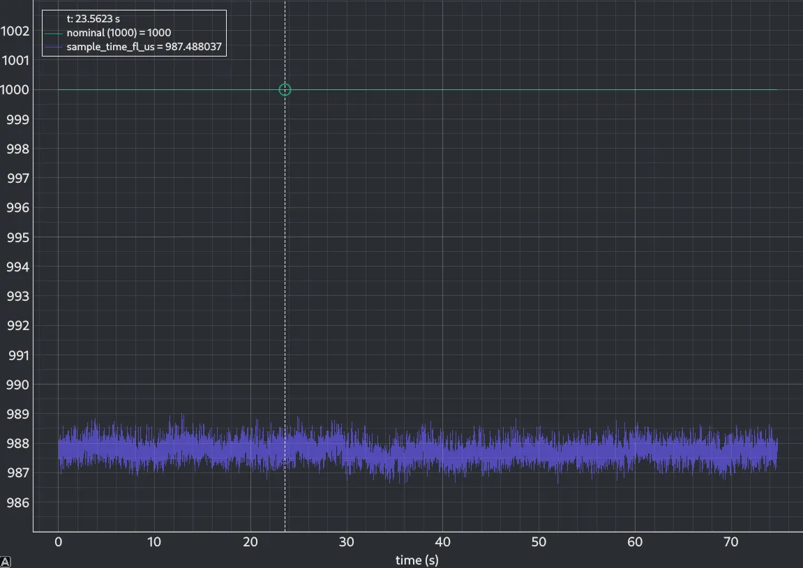Figure 3 — Initial timing measurement, with the sensor on its default internal oscillator. The trace sits about 12 µs below the nominal (1000) line and wanders across roughly two microseconds; the cursor reads one sample at 987.5 µs, and the mean over all 41,729 is 987.7.

A little over one percent is small enough to dismiss and large enough to matter. It is a rounding error in a control loop and a serious problem in an integral. At this point, simply reporting the measured number would not be enough. The interesting question became:

What is causing the discrepancy?

Investigating the Clock Source

The MPU6050 does not derive its internal sampling timing from the STM32 clock. It has its own internal clocking system, including a selectable clock source, and SMPLRT_DIV divides that internal clock down to the output rate. The divider is exact. The clock being divided is not necessarily what you assume.

The initial configuration used the MPU6050’s default source, which is an internal 8 MHz relaxation oscillator — cheap, always available, and not built to be a frequency reference. The register map is unusually direct about this and recommends selecting a gyroscope PLL instead, which ties the sensor’s timing to the gyroscope’s own resonator.

So the CLKSEL field of PWR_MGMT_1 was changed from 0x00 to 0x03, selecting the PLL referenced to the Z gyroscope. Any of the three gyroscope references will do — 0x01, 0x02 and 0x03 select X, Y and Z, and the bring-up article picks X.

The STM32 clock and the DWT timing reference were not changed. Neither was the sample rate divider, the low-pass filter, or either full-scale range.

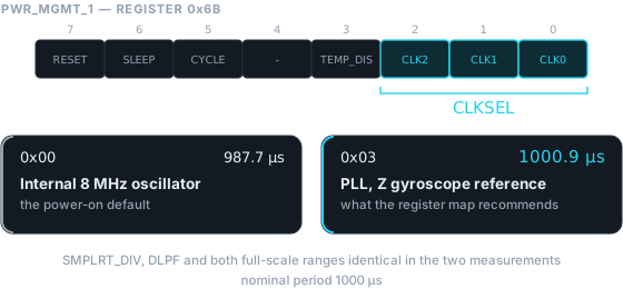Figure 4 — MPU6050 clock-source configuration using the gyroscope PLL. The sample rate divider was identical in both measurements; only the clock it divides changed.

After repeating the measurement with the same 1 kHz sensor configuration, the measured period moved to 1000.9 µs — 999.1 Hz, within 0.1 % of nominal. The sample-to-sample variation improved at the same time, and by more: the standard deviation of the interval fell from 271 ns to 27 ns, a factor of ten.

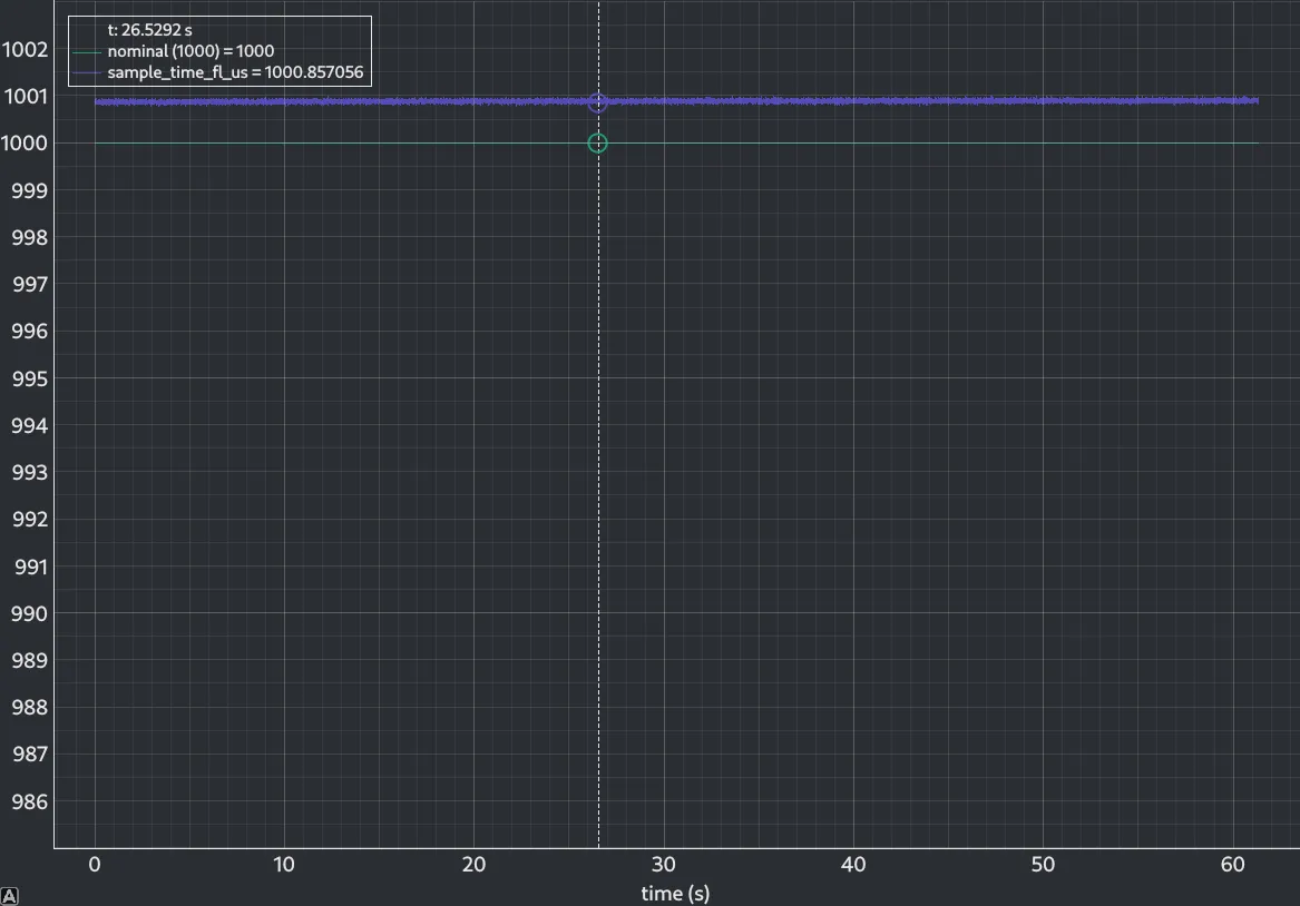Figure 5 — The same axes and the same channels as figure 3, with one register value different. The interval lands on the nominal line and the band collapses to a fraction of its former width; the cursor reads one sample against a mean of 1000.89 µs over all 32,114.

Nothing changed on the board but that one register, and temperature cannot account for the shift. Four PLL captures spanning 30.6 to 33.9 °C agree within 0.06 µs of each other. Over much the same interval the internal oscillator moved 2.36 µs, from 990.1 µs at 31 °C to 987.7 µs at 33 °C. It drifts about forty times further with temperature than the PLL does.

And the change of clock source moved the period 13.1 µs. That is two hundred times the PLL’s own drift, so there is nothing else it could be.

Those are raw movements between captures, not a fitted coefficient, and none is offered here. But the bring-up article’s “measurably more stable over temperature” is now a number rather than a claim.

This was a particularly useful result, because it showed that the observed timing was not a property of the STM32 measurement system. The sensor configuration had not changed from 1 kHz. The STM32 timing reference had not changed. The internal clock source of the MPU6050 had changed — and the measured sampling period changed with it.

This is also where the bring-up article’s one-line recommendation came from. It was written as a stability argument, and the frequency error above is the rest of the reason. The write has been in the firmware ever since, so every published capture in this series was taken on the PLL and no earlier result moves. The gyroscope article measured the sensor at 999 Hz over 961,000 samples on two independent clocks, which agrees with 1001 µs to better than a tenth of a percent.

The uncomfortable part is what it would have cost to leave alone. A 1.2 % error in the sample period is not visible in a sensor reading and trips no check. It also survives a full calibration, because a calibration that uses the wrong dt on both sides of its arithmetic just folds the error into its own constants.

The Corrected Measurement

After switching to the gyro PLL clock source, the sampling period was very close to the expected 1 ms. In microseconds, the result looks remarkably stable:

1001 µs    1001 µs    1001 µs    1001 µs    ...

That is not an abbreviation. Rounded to whole microseconds, all 32,114 samples in the capture reported 1001, and nothing else — minimum 1001, maximum 1001, standard deviation exactly zero.

At first glance it would be tempting to conclude that there is essentially no jitter. But that conclusion would be premature. We have only looked at the measurement with microsecond resolution.

What happens if we look closer?

Part 2 — How Much Jitter Is Really There?

Measurement Resolution Matters

The same measured interval can be expressed in microseconds, in nanoseconds, or in raw CPU clock cycles. All three represent the same physical interval, but they do not reveal the same amount of detail.

At microsecond resolution, several slightly different measurements collapse into the same displayed value. For example:

1000.7 µs    1001.1 µs    1001.4 µs    1001.8 µs

may all appear as approximately 1001 µs. Inspect the raw cycle count instead and those differences become visible.

The firmware measures the interval once, in cycles, because that is what the counter produces. It then exports the same number three ways: raw cycles, whole microseconds, and microseconds as a floating-point value. All three describe one event.

Choosing which of them to look at is a workspace decision in EmbedStudio rather than a rebuild, and a histogram there counts whatever range a scope hands it. So both of the figures below are the same capture over the same samples. Only the ruler differs.

The Microsecond View

The histogram in microseconds shows a very tight distribution. Most measurements fall within approximately one microsecond of the central value. It looks almost like a single solid peak.

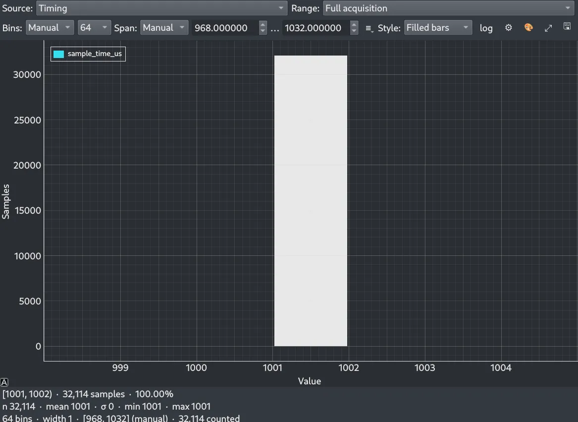Figure 6 — The interval in whole microseconds, over a 64 µs wide axis. Every one of the 32,114 samples falls in the same bar, and the panel reports minimum 1001, maximum 1001 and a standard deviation of zero.

From a practical perspective, this is an excellent result. For many applications, sub-microsecond variation is completely irrelevant. But the measurement contains more information than this histogram shows.

Looking at the Cycle Counter

Now we change only the representation. Instead of displaying the interval in microseconds, we display the number of CPU cycles between consecutive DATA_RDY events. The underlying measurement has not changed. Only the resolution has changed.

And suddenly the distribution is no longer a single solid peak. It is a bell. The same 32,114 samples that took one value in microseconds take 28 distinct values in cycles.

The reason is a mismatch of scale. At 168 MHz one microsecond is 168 cycles, and the real variation here spans about 22 cycles — roughly an eighth of the rounding step. Anything that much narrower than the ruler cannot survive being measured with it.

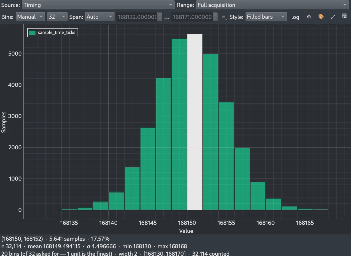Figure 7 — The same 32,114 samples, counted in core clock cycles instead. The single bar resolves into a distribution centred on 168,149 cycles with a standard deviation of 4.50 — 27 nanoseconds, and about an eighth of the microsecond that hid it.

This is an important lesson:

The absence of visible jitter does not necessarily mean the absence of jitter. It may simply mean that the measurement resolution is too coarse to reveal it.

Neither view is more “correct” than the other. Figure 6 answers “is this good enough for my control loop”, and the answer is yes with room to spare. Figure 7 answers “what is actually happening”, which is the question you need when something later does not add up.

What Does the Jitter Actually Mean?

It is tempting to look at the cycle-level histogram and conclude that every variation represents a problem. That would also be incorrect.

A real digital system contains many sources of small timing variation. The MCU clock is not an infinitely precise mathematical reference. Interrupt entry takes a variable number of cycles. The sensor’s internal timing and the MCU clock are not locked to each other.

The important question is therefore not:

“Is every sample exactly the same number of CPU cycles apart?”

but rather:

“Is the timing variation small enough for the intended application?”

For the MPU6050, the answer after correcting the sensor clock configuration is clearly much better than the initial measurement suggested.

Part 3 — Can We Trust the Measurement?

The Timestamp Is Taken Inside an Interrupt

There is another subtlety. The DATA_RDY signal causes an interrupt, and the timestamp is obtained while servicing that interrupt, so the measurement is not completely independent of the MCU’s interrupt system.

The hardware DATA_RDY event occurred at one moment. The timestamp is captured later, once the core has finished whatever it was doing, entered the handler and reached the instruction that reads the counter. Normally that is a fixed, small number of cycles and it cancels out of the subtraction entirely.

It stops cancelling if something delays entry. This is normally a very small effect. At microsecond resolution it may be invisible. At cycle resolution, however, it can become measurable.

Why Interrupt Priority Matters

This is easy to test, because it is a property of the configuration rather than of the hardware. Build the firmware twice, changing nothing but which of the two interrupts outranks the other, and capture the same 61 seconds each way.

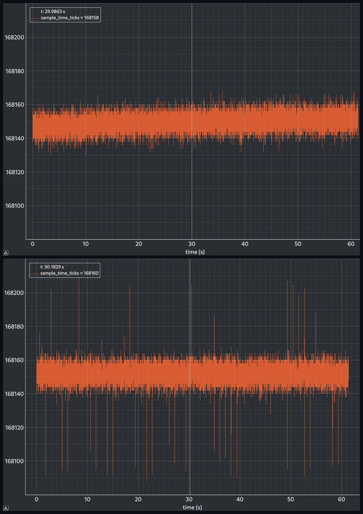Figure 8 — The same firmware, the same board, the same minute of sampling. Above, the data-ready interrupt outranks SysTick and the interval never leaves a twenty-cycle band. Below, the two are swapped, and a tick arriving at the wrong moment pushes the timestamp out by up to sixty cycles.

The lower trace is not noisier everywhere. Its band is the same width as the one above it, and the excursions are 33 events in 32,454 samples — one sample in a thousand. Each is about 55 cycles, or 330 ns.

Two details identify the cause beyond doubt. Where both halves were captured the spikes come in pairs of opposite sign, a long interval and then an equally short one, which is what a delayed timestamp looks like as opposed to a genuinely different sampling interval. And they are not random in time: they arrive every 1.11 seconds. SysTick runs at exactly 1000 µs and the sensor at 1000.9, so the two drift through coincidence at 0.902 Hz — one collision every 1.109 seconds. That is the cadence in the figure, predicted before it was measured.

The important lesson here is broader than the MPU6050:

A high-resolution timer does not automatically make a measurement high-accuracy. The measurement mechanism itself can influence what is being measured.

The practical rule follows directly. If a measurement is taken inside an interrupt, that interrupt has to outrank everything that is allowed to interfere with it. Here that is one line of firmware, it costs nothing, and the upper trace in figure 8 is what it buys.

There is a trap in how priorities are applied, and it cost a wasted afternoon here. Setting a priority is not enough on its own, because the number is interpreted against the current priority grouping, and the grouping decides how many of the bits mean pre-emption at all. This project was generated with NVIC_PRIORITYGROUP_0, which allocates none of them. Under that grouping nothing can pre-empt anything, and the priority numbers only decide which of two already pending interrupts is served first.

So a priority set under it looks entirely correct and does nothing at all. Both configurations above needed the grouping set as well as the numbers, and the firmware linked at the end of this article now does exactly that — it selects NVIC_PRIORITYGROUP_4 and then assigns both priorities explicitly, rather than inheriting whatever the generated code left behind.

Interrupt latency deserves more than this, and it applies to any interrupt-driven sampling system rather than to this sensor, so the general treatment belongs in a note of its own.

Why Not Simply Use the Average?

At this point we have several different pieces of information:

• nominal sampling rate: 1 kHz, i.e. 1000 µs;
• initial measured period: 987.7 µs, an effective 1012.4 Hz;
• corrected measured period: 1000.9 µs, an effective 999.1 Hz;
• interval variation: 271 ns before the change, 27 ns after it;
• microsecond-resolution distribution: a single bar;
• cycle-resolution distribution: 28 distinct values across about 22 cycles.

A single average value would hide most of this story. That is why timing analysis should look at both the central value and the distribution around it.

Why Does dt Matter?

The timing experiment would be little more than an interesting measurement if timing had no effect on the algorithms that process the sensor data. It does.

Consider gyroscope integration. Angular velocity is measured in degrees per second, and to obtain an angle we integrate it over time:

angle[n] = angle[n-1] + gyro[n] × dt[n]

If we simply assume dt = 1 ms for every sample, we are assuming the sampling interval is perfectly constant. But we have just demonstrated that the actual interval can differ from the nominal value. If the true interval is 987.7 µs and the firmware assumes 1000, every angle it computes is 1.2 % too large, and it grows without limit for as long as the integration runs.

For scale: the previous experiment measured one gyroscope axis at 0.9 % above its nominal scale factor and treated that as worth an article. An unmeasured clock source is the same size of error, applied to every axis at once and in the same direction — and it costs one byte to remove rather than a calibration session.

If the firmware has measured dt[n], it can simply use that actual value. This removes the need to pretend that every sample took exactly the same amount of time.

Timing and Frequency Analysis

Timing also matters for frequency analysis, where the sampling frequency is related to the sample period:

Fs = 1 / dt

If the actual sampling period differs from the nominal value, the effective sampling frequency differs as well. A 1.2 % error in dt puts a 1.2 % error on every frequency in the result — a vibration at 100 Hz reads as 101.2 Hz. No amount of resolution in the transform fixes it, because the error is in the axis rather than in the data.

Again, the nominal configuration tells us what we asked the system to do. The measured timing tells us what the system actually did.

Timing and Sensor Fusion

The timing information becomes even more important when the accelerometer and gyroscope are combined into an IMU.

A sensor-fusion algorithm does not only need sensor values. It also needs to know how much time has elapsed between updates, because that is what sets how much it trusts the integrated rate before pulling it back towards gravity. Feeding it a constant while the real interval differs puts a systematic error into the tuning of the filter itself, which is a much harder thing to debug than a wrong constant.

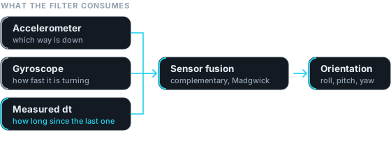Figure 9 — Accelerometer data, gyroscope data and the measured dt entering the future sensor-fusion stage. The interval is a third input of equal standing, not a constant baked into the filter.

This is why timing is worth investigating before building the complete IMU. It gives us confidence that the dt supplied to the algorithm is a measured quantity rather than an assumption.

The Timing Module

The DWT-based timing functionality used in this experiment is implemented as a reusable module in the project. It initialises the cycle counter, caches the core clock frequency, and provides timing information at different resolutions — nanoseconds, microseconds, milliseconds, seconds, and the underlying clock-cycle count. Cycles stay the primary representation, and a conversion happens only when a human needs to read the value.

It has no dependencies beyond CMSIS. It uses no timer peripheral, no SysTick, no interrupt and no RTOS, which is what makes it safe to call from inside a handler and from inside the code being measured. It is useful not only for measuring sensor timing, but also for measuring firmware execution time and investigating other timing-related problems.

The implementation and API are intentionally not covered in detail here. A separate article will describe the module itself, including:

• how the DWT cycle counter works;
• initialization;
• time conversion;
• available measurement resolutions;
• API usage;
• execution-time measurements;
• practical limitations.

The module is available in the project repository for anyone who wants to reuse it.

Conclusion

A sensor configured for 1 kHz does not automatically mean that every observed sample interval will be exactly 1000 µs. This experiment showed several layers of the problem.

First, the initial measurement revealed a surprisingly large deviation, 987.7 µs, despite the nominal 1 kHz configuration. Investigating the MPU6050 clock configuration led to switching its internal clock source to the gyro PLL. The STM32 clock and DWT timing reference were not changed. After that change, the measured period moved to 1000.9 µs, and the interval variation fell from 271 ns to 27 ns.

Then we looked more closely at the measurement. At microsecond resolution, the sampling period appeared almost perfectly stable. At CPU-cycle resolution, small variations that had been hidden by the coarse representation became visible.

Finally, we saw that even a high-resolution measurement has its own limitations. Interrupt latency and interrupt priority can influence when the timestamp is actually captured.

The main lessons are therefore:

• a nominal sample rate is not the same as a measured sample period;
• the MPU6050’s internal clock-source selection can significantly affect its actual sampling timing, and the fix is one byte written once at bring-up;
• measurement resolution determines which timing variations are visible;
• high-resolution measurements can reveal effects hidden at lower resolution;
• interrupt latency can influence measurements made inside interrupt handlers, and giving the measurement the higher priority removes it;
• measured dt can be used directly by time-dependent algorithms.

The most important principle is simple:

If an algorithm depends on time, measure time instead of assuming it.

The measurement itself was cheap. The firmware records a cycle count per sample and does nothing else with it. Everything after that happened in EmbedStudio, against a recording that was already on disk — switching the histogram from microseconds to cycles was a change of channel, not a rebuild.

With the sensor calibrated and its timing understood, the next step is to look at what the numbers underneath are actually made of.

References

• InvenSense, MPU-6000 and MPU-6050 Register Map and Descriptions, Rev. 4.2 (RM-MPU-6000A-00, 2013) — PDF. Source of the PWR_MGMT_1 clock-select field, and of the recommendation to run the device from a gyroscope reference rather than its internal oscillator.
• Arm, ARMv7-M Architecture Reference Manual — the Data Watchpoint and Trace unit and its CYCCNT cycle counter, the timing reference used throughout.

Next Experiment

Experiment #005: How Noisy Is the Signal Underneath?

The interval between samples is measured now, and the values arriving at each of those instants are calibrated. What has not been characterised is the part of each reading that is neither signal nor bias. That is the noise: its size, its shape, and how much of it a filter can remove before it starts removing the measurement as well.

That question needs a trustworthy time axis before it can even be asked, which is why it comes after this one. The point of looking at noise is to find where in the band it lives. A spectrum computed against a sample rate that is 1.2 % wrong puts every one of those frequencies in the wrong place.