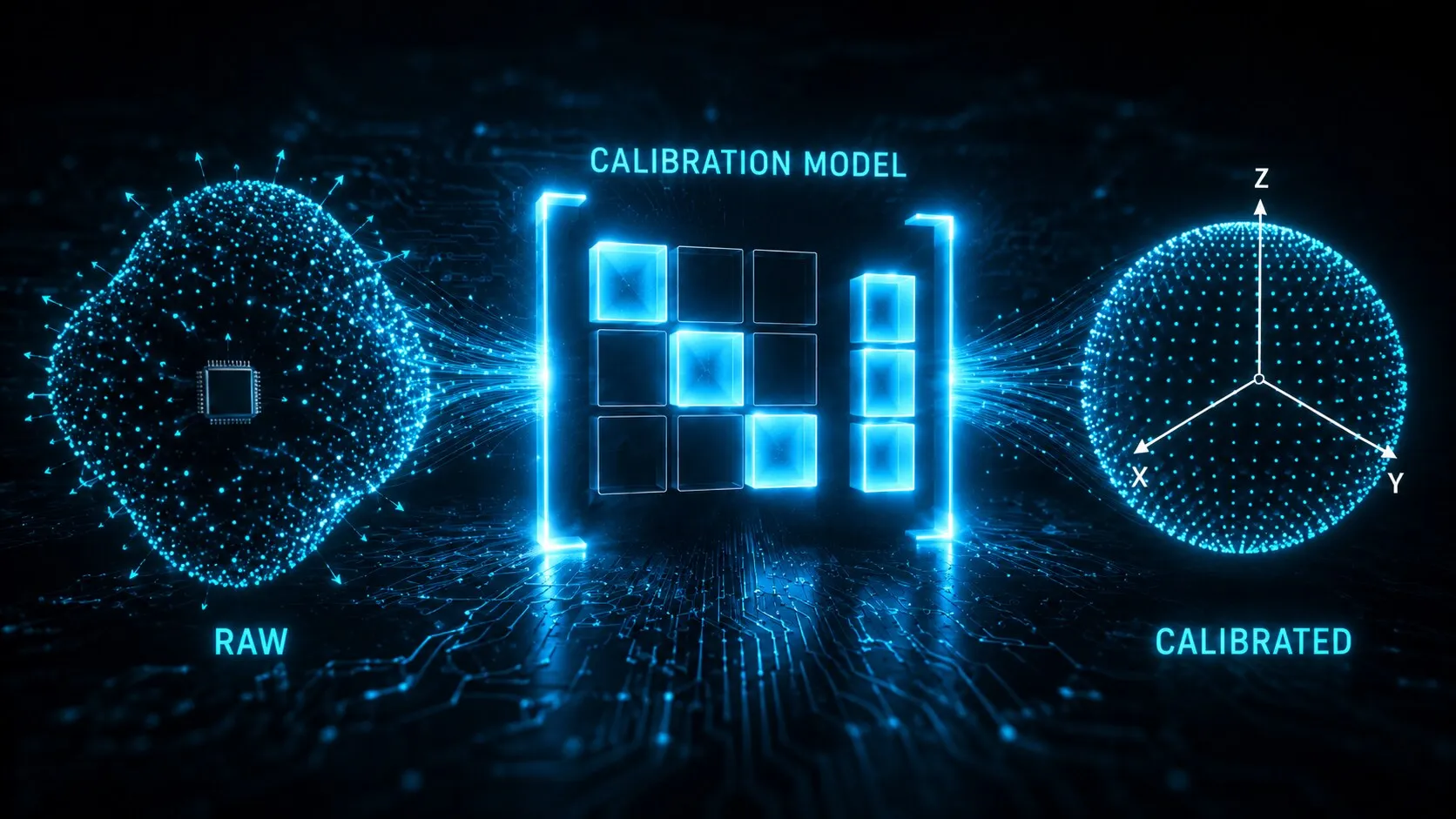
MPU6050 Accelerometer Calibration: Six-Position Method on STM32

Lay our MPU6050 flat on a table and it reports 1.012 g. Gravity has not changed — the sensor is wrong, by 1.2%, straight out of the bag.

Manufacturing tolerances leave three errors in the raw counts: an offset that shifts every reading, a gain error that scales it, and noise that makes it wobble. Calibration fixes the first two, and the fix is one line per axis:

acceleration[g] = (raw - bias) / scale

Six constants, then. The interesting part is getting them — with no jig, no rotary stage and nothing but gravity as a reference — and then finding out how long they stay true.

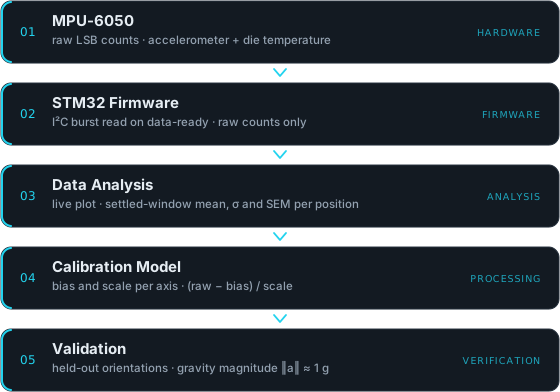Each stage produces the input to the next; the calibration constants are only written into firmware after validation.

What this experiment found

• Six static positions, each a short steady hold, are enough to measure bias and scale for all three axes — hand-held, no jig, no rotary stage, no machined reference surface.
• Uncalibrated, this module was out by up to 1.9% on gravity magnitude. Calibrated, 0.68% at orientations it had never been calibrated at.
• Scale factors are stable; offsets are not. Scale reproduced to 0.03% across a power cycle; bias moved by up to 2.2 mg. The two constants have different shelf lives, and firmware should treat them as such.
• Validating only at the six calibration positions would have reported 0.24% and been misleading — a model reproduces its own fit points by construction.

1. Hardware and Firmware Setup

Hardware

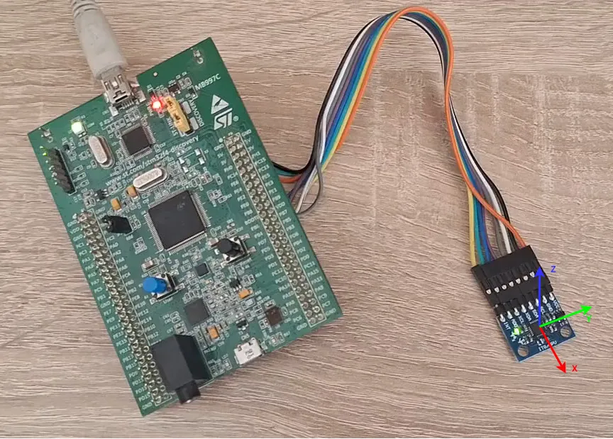The axis arrows on the module — X red, Y green, Z blue — define every orientation used below; the six positions in section 3 are named after them.

Setup components and interconnections are described in Experiment #001.

Firmware

The firmware does two things: initialise the MPU6050, and read a sample when the data-ready interrupt fires. No calibration — that comes later, and only once the constants have been proven.

Five registers set up the measurement, and the numbers in this article cannot be read without them:

Register	Addr	Value	Why this value
PWR_MGMT_1	0x6B	0x03	Clears SLEEP; CLKSEL = 3 → PLL with Z-axis gyro reference
CONFIG	0x1A	0x03	DLPF_CFG = 3 → ~44 Hz accelerometer bandwidth, 1 kHz base rate
SMPLRT_DIV	0x19	0x00	Output data rate = 1 kHz / (1 + 0) = 1 kHz
ACCEL_CONFIG	0x1C	0x00	AFS_SEL = 0 → ±2 g full scale, 16384 LSB/g nominal
INT_ENABLE	0x38	0x01	DATA_RDY_EN — every sample is taken on the data-ready interrupt

Two traps before you copy that table:

• The DLPF changes the sample rate. SMPLRT_DIV divides a 1 kHz base rate with the filter on, and an 8 kHz base rate with it off. Disabling the filter multiplies your output rate by eight without touching the divider.
• The full-scale range fixes the nominal sensitivity. ±2 g means 16384 LSB/g, which is what we compare the measured scale factors against in section 5. At another range it is another number.

We leave the 44 Hz bandwidth alone. A calibration capture averages thousands of static samples, so the averaging is the real low-pass filter here.

2. What Causes Accelerometer Error: Bias, Scale and Noise

Back to that flat board. Here is what it should read, and what it actually reads:

Axis	Ideal output	Real measurement
X	0 g	0.012 g
Y	0 g	−0.004 g
Z	1 g	1.012 g

Three axes, three errors, all of them small and none of them zero. The model behind them is deliberately simple — bias shifts the reading, scale stretches it:

raw = scale * true_value + bias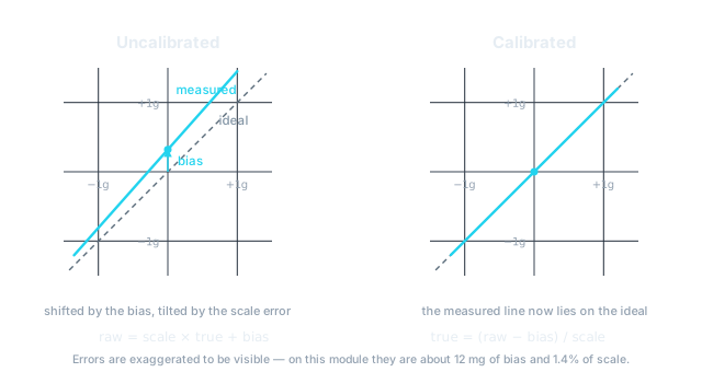

Bias offsets the response, scale tilts it. Calibration removes both, leaving the measured output on the ideal line.

Temperature

Both constants drift with temperature, so let the board warm up before capturing anything — calibrate a cold part and you get constants for a cold part.

Checking costs nothing, because the MPU6050 reports its own die temperature in the same burst transfer as the acceleration data. Don’t read it as room temperature: it is inaccurate in absolute terms and the die runs warmer than the air around it. But it resolves changes well, which is all we need to tell a settled sensor from a still-warming one.

So temperature is recorded next to every table below. Quantifying its effect needs a controlled heat soak, and gets its own experiment later in this series.

3. The Six-Position Calibration Method

Calibration needs a reference of known magnitude, and there is a free one in the room: gravity is 1 g, everywhere, always, and it costs nothing to borrow.

Point each axis up, then down. That gives a +1 g and a −1 g reading on all three axes — six numbers, which is exactly enough to solve for six constants.

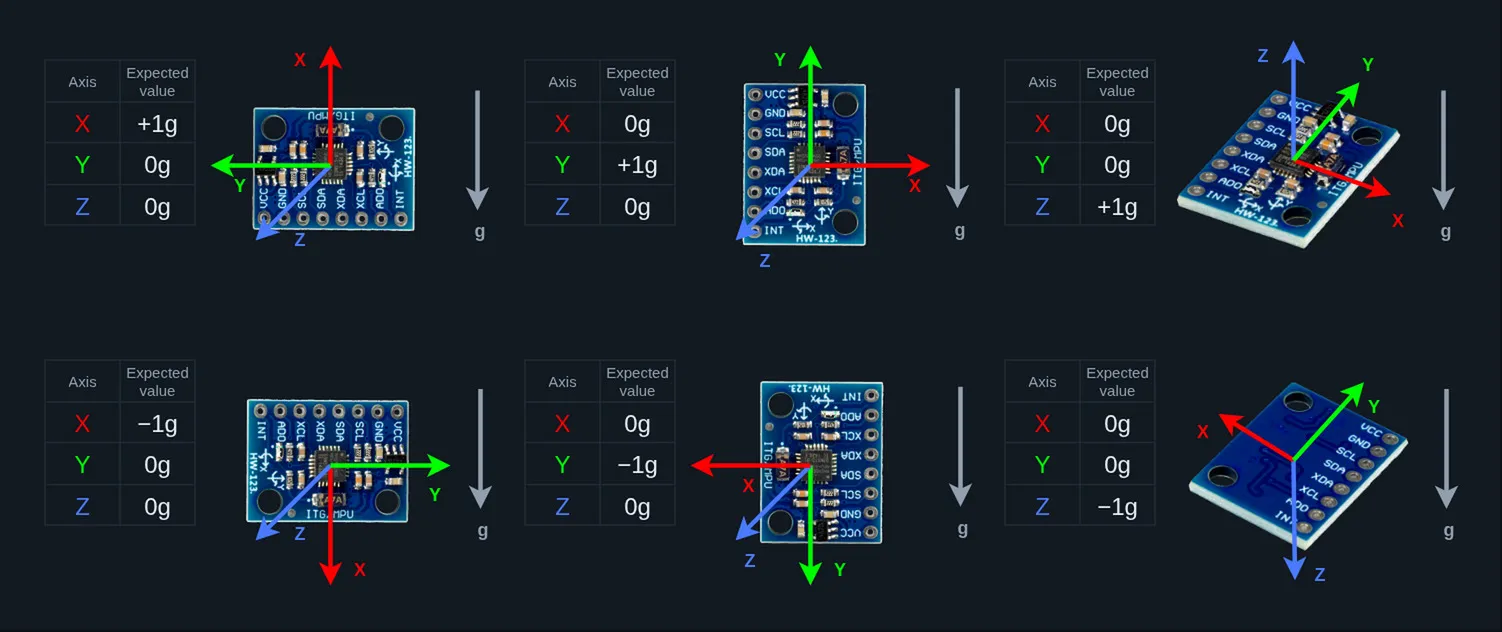Each axis is pointed up, then down. An accelerometer senses the reaction to gravity, so the axis pointing up is the one reading +1 g. Axis colours match the arrows on the photograph in section 1.

4. How to Position the Sensor Without a Jig

Don’t try to position the board accurately. Read the position off the data instead: one axis near ±1 g, the other two near zero. This is +X —

Accel X = 1.03g
Accel Y = 0.01g
Accel Z = -0.02g

— and it does not matter that the board is nowhere near square with anything.

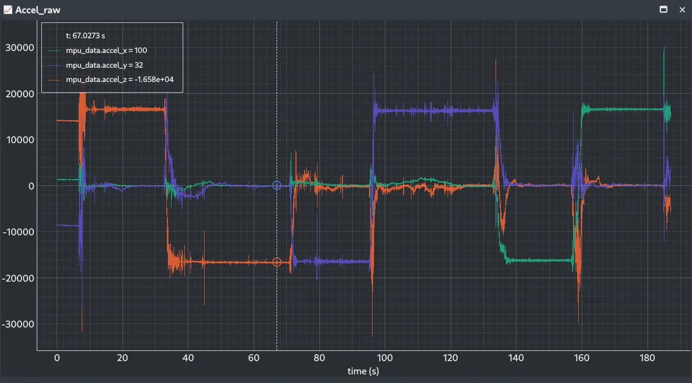Raw accelerometer measurements during the calibration procedure.

Aligning by nulling the orthogonal axes

The module is a bare PCB with no machined reference surface, and we used no jig and no rotary stage — the board was held by hand throughout, neither clamped nor rested on a surface. Adjust it until the two orthogonal axes read close to zero on the live plot, and only then capture.

That works because the two axes behave completely differently near alignment. If the board is off by an angle ε, the dominant axis reads cos ε while an orthogonal axis reads sin ε:

Misalignment ε	Orthogonal axis (sin ε)	Error on dominant axis (1 − cos ε)
0.5°	143 LSB	0.6 LSB (0.004%)
1.0°	286 LSB	2.5 LSB (0.015%)
2.0°	572 LSB	10 LSB (0.06%)

That table is the whole trick. The orthogonal reading grows with ε; the error it causes on the dominant axis grows with ε². A 1° misalignment is plainly visible as a ~286 LSB orthogonal signal — far above the sample noise — yet it corrupts the scale factor by only 2.5 LSB out of 16384. The indicator is around a hundred times more sensitive than the error it is guarding against, so no reference hardware is needed.

That is also why a hand is good enough. Holding the board steady to within a degree is easy; holding it to within a degree of a known direction is not, and nulling never asks for the second. A live plot and a pair of hands is the entire tooling requirement, so the same six positions can be run on a device already in the field.

Nulling has one more advantage: it aligns gravity to the sensor’s own axes rather than to the PCB edges or the table, so die-to-package mounting tolerance gets absorbed along with everything else. A perfectly square fixture would not correct that.

Optional second pass. The value being nulled still contains that axis’s own bias, so nulling it to zero leaves a small real tilt of asin(bias / scale) — under 0.7° for the offsets measured here. If you want it gone, run the six positions once, compute preliminary biases, then repeat while nulling the bias-corrected values. Only the first pass was run in this experiment: 0.7° of tilt shifts the dominant axis by about 1.2 LSB, which is smaller than the uncertainty on the calibration points themselves.

5. Calculating Bias and Scale from the Measurements

Everything here stays in raw LSB. One axis gives two readings, and two readings are enough to solve for two unknowns:

raw+ =  scale + bias        (axis up)
raw- = -scale + bias        (axis down)

bias  = (raw+ + raw-) / 2   midpoint of the two
scale = (raw+ - raw-) / 2   half the distance between them

That is the standard two-point construction, not something invented for this experiment — Analog Devices’ AN-1057 derives the same per-axis model, just in g rather than raw LSB.

Capture protocol

The sensor configuration is the one from section 1. The capture itself:

Each position was found by nulling the two orthogonal axes, and most of the time per position went on that alignment rather than on the capture. Once the readings settled, the analysis window was chosen as the stretch where the two orthogonal axes deviated least — between 8399 and 14070 samples per position.

Picking the window that way applies section 4’s null criterion to the data instead of to the board. Alignment is the one error source you can still reduce after the capture is over, and it costs nothing to do.

Per-position statistics

Position	N	Mean (LSB)	σ (LSB)	SEM (LSB)	T (°C)
+X	14070	16605.1	94.2	0.79	29.8
−X	13583	−16210.4	113.2	0.97	29.4
+Y	9989	16331.0	141.3	1.41	29.3
−Y	8930	−16471.5	141.2	1.49	28.9
+Z	9584	16573.7	149.9	1.53	27.8
−Z	8399	−16648.7	65.2	0.71	28.6

SEM = σ / √N is the standard error of the mean as the analysis panel computes it. It assumes every sample is independent, which these are not, so treat it as a lower bound on the uncertainty of each calibration point rather than the uncertainty itself. T is the mean die temperature during the capture.

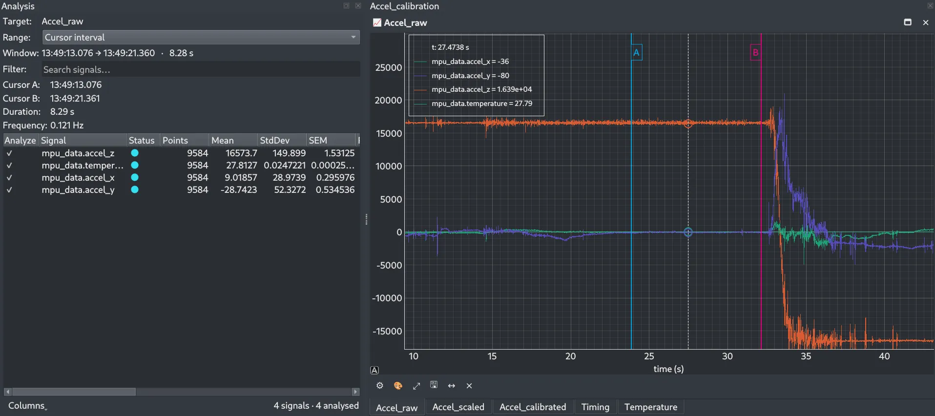Where those numbers come from — a cursor-bounded window on the left, and per-signal mean, σ and SEM on the right. This is the +Z capture, the fifth row of the table above.

Two things in that table are worth a second look.

σ is not the sensor’s noise — it is yours. It ranges from 65.2 LSB in the −Z position to 149.9 LSB in +Z, a factor of 2.3 between two orientations of the same axis. Intrinsic sensor noise cannot do that; it would be the same in every position. What changes is how steadily the board can be held in a given orientation. In absolute terms σ spans roughly 4 to 9 mg — and it is mostly a measure of the hand holding the module.

The averaging still wins. Consecutive samples through the 44 Hz filter are correlated, so the honest error on each mean is about 3.4× the naive σ/√N — 2.4 to 5.2 LSB. That puts each bias at roughly ±2 to ±3.5 LSB, far smaller than the biases themselves. Remember that number: section 7 shows the offsets moving about ten times that much between power cycles.

Averaging ten thousand samples is what makes a shaky hand good enough. If you need a calibration point pinned down tighter, hold the position longer — changing the filter does not help, because it raises σ and the useful sample count together.

The six means above are the inputs to the bias and scale calculation:

Axis	+1g raw	−1g raw	Bias (LSB)	Bias (mg)	Scale (LSB/g)
X	16605.1	−16210.4	197.35	+12.0	16407.75
Y	16331.0	−16471.5	−70.25	−4.3	16401.25
Z	16573.7	−16648.7	−37.50	−2.3	16611.20

These constants belong to this module, at this temperature. They were measured across a die temperature of 27.8–29.8 °C and are only valid near it — don’t copy them into your own project.

The datasheet’s nominal sensitivity at ±2 g is 16384 LSB/g. Against that, this part deviates by:

Axis	Scale (LSB/g)	Nominal (LSB/g)	Sensitivity error
X	16407.75	16384	+0.15%
Y	16401.25	16384	+0.11%
Z	16611.20	16384	+1.39%

X and Y sit within 0.15% of nominal; Z is out by 1.39%, roughly ten times more. Z is also the axis that spends most of its time pointing at gravity in a stationary device, so that one deviation dominates the uncalibrated error: the −Z position reads 1.62% high before correction, against 0.32% for +Y. That is where the “why does my flat board read 1.012 g” from section 2 comes from.

The scale factors are also the stable half of this calibration — measured again after a power cycle they reproduce to within 4.5 LSB, while the biases move nearly ten times as much. That split matters more than either value on its own, and section 7 comes back to it.

6. Testing the Model Before Writing Any Firmware

The model is six constants and two operations per axis — simple enough to look finished and still be wrong. A sign error, or an axis paired with another axis’s scale factor, produces output that looks perfectly plausible and is quietly incorrect.

Build, flash, re-measure is a slow way to find that out. So we ran the model as a processing chain over the live data in EmbedStudio instead — three raw channels in, (raw − bias) / scale per axis, and the magnitude derived from the results:

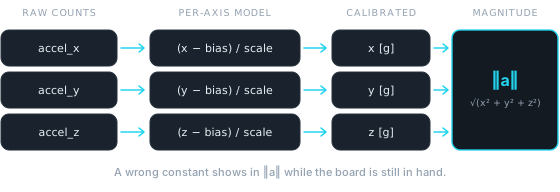The calibration model evaluated as a signal processing chain, before any of it exists in firmware. The magnitude is derived alongside the raw channels, which is what makes a wrong constant visible live.

Two things follow from working this way. Changing a constant becomes an edit instead of a rebuild — the six-position fit, the repeat run after a power cycle and the twelve poses in section 7 all go through the same chain with different numbers in it. And because the magnitude is computed alongside the raw channels, the pass/fail criterion is visible while the board is being moved. Watching ‖a‖ hold at 1 g through a slow tilt catches a wrong constant faster than any amount of post-processing.

The firmware still reads raw counts and nothing else. The constants only move into it in section 9, once they are known to work.

7. Validating the Calibration

A calibration has to be checked against measurements that were not used to build it. The check is easy, because gravity is the same size whichever way you turn the sensor — so for a board held still, this should come out at 1 g and stay there:

magnitude = sqrt(x² + y² + z²)   →   ≈ 1 g

Repeating the six positions

The first check repeats the six orientations with a new capture, constants held fixed at the values found above. Nothing is refitted.

Running the model over the same data it came from would prove nothing — each dominant axis returns exactly ±1.000 g by construction. Do that once as a wiring check on the processing chain, and no more.

A fresh capture is a different matter. The board was power-cycled, repositioned, re-nulled and re-acquired, so any deviation from ±1.000 g now means something real: positioning repeatability, plus whatever the bias has done since.

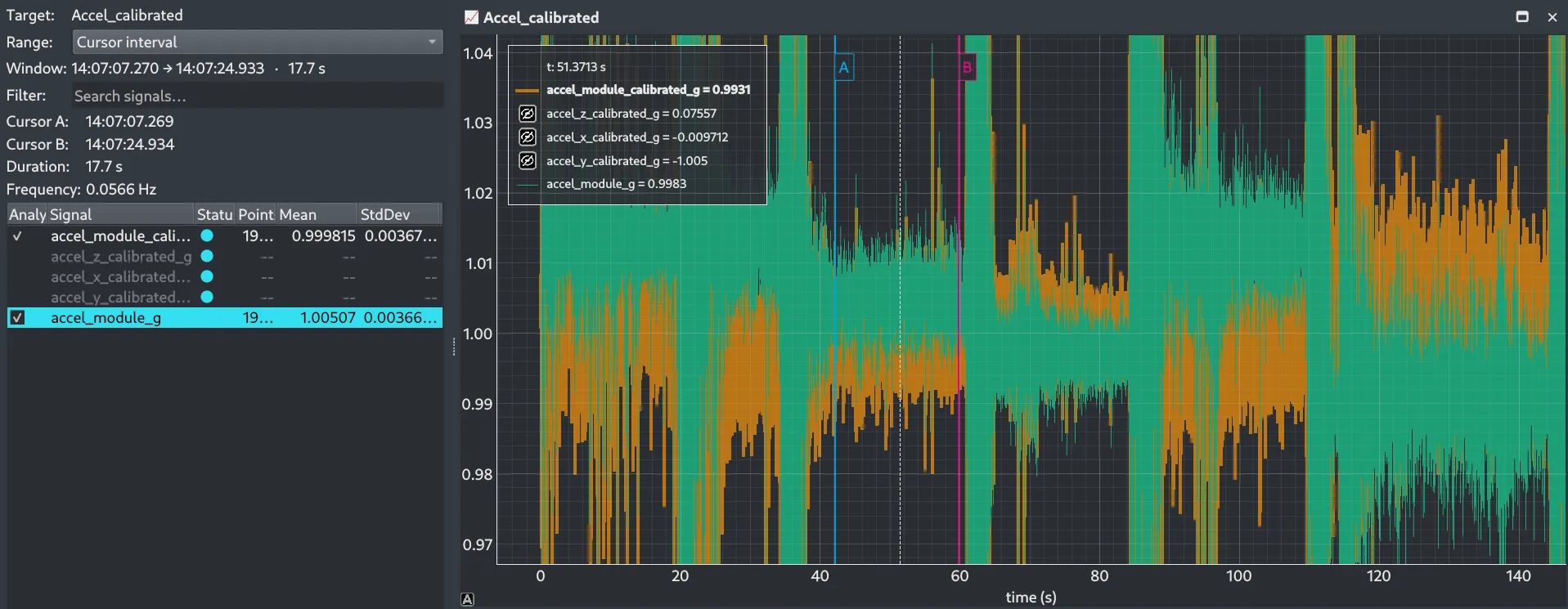The repeat capture as gravity magnitude. Over the 17.7 s between the cursors the calibrated trace averages 0.9998 g against 1.0051 g uncalibrated; the full-height bands are the board being moved between positions.

Position	‖a‖ error, uncalibrated	‖a‖ error, calibrated	T (°C)
+X	+1.278%	−0.070%	30.8
−X	−0.930%	+0.128%	31.1
+Y	−0.332%	−0.003%	30.6
−Y	+0.523%	−0.011%	29.8
+Z	+1.365%	+0.209%	28.6
−Z	+1.364%	−0.244%	28.9

The uncalibrated column applies the datasheet’s nominal 16384 LSB/g with no offset; the calibrated one applies the constants from section 5.

Since the constants came from the earlier run, the calibrated column is not a residual in the usual sense — it is the drift accumulated since calibration. Recomputing bias and scale from this run and differencing them against the stored values splits that drift into a shift of the zero point and a change in sensitivity:

Axis	Δ bias (LSB)	Δ bias (mg)	Δ scale (LSB)	Δ scale (%)
X	−16.40	−1.00	+4.50	+0.027
Y	+0.35	+0.02	−1.85	−0.011
Z	+37.30	+2.25	−4.10	−0.025

The two parameters behave completely differently, and that is the main result of this experiment.

Scale is stable. Across a power cycle and a full repositioning of the board, every scale factor came back within 4.5 LSB of its stored value — better than 0.03% on all three axes. Whatever changes between sessions, the sensitivity does not.

Bias is not. The Z offset moved by 37 LSB (2.25 mg) and X by 1.00 mg — an order of magnitude more than the scale drift, and about ten times the ±2 to ±3.5 LSB precision the calibration itself achieved. All that care spent pinning each calibration point to a couple of LSB is undone by switching the board off and on again. (The Y bias moved 0.35 LSB, which is nothing; only the X and Z shifts are large enough to be certain of.)

So the two deserve different treatment: the scale factors are worth storing, the offsets are worth re-measuring. An offset measured today does not describe the device tomorrow, which is why production systems re-zero on boot instead of trusting a stored constant. Section 9 weighs that against what a measurement rig actually needs.

One caveat this table cannot settle: the repeat run sat about 1 °C warmer than the calibration run (28.6–31.1 °C against 27.8–29.8 °C), so some unknown part of the bias shift is thermal rather than turn-on.

This table is also the diagnostic one. Each row isolates a single axis, so it tells you which axis is misbehaving and whether the fault is in the offset or the sensitivity. The magnitude test below can do neither.

Magnitude at arbitrary orientations

Repeating the calibration positions can expose an unstable model, but not an inadequate one. Errors the diagonal model cannot represent only show up where all three axes carry signal at once — never at a pose where one axis holds the whole gravity vector.

So we held the board in twelve arbitrary static orientations that were not used to fit the parameters, several of them loading every axis to roughly 0.5 g, and averaged the magnitude at each.

This is the easiest test in the article to run: ‖a‖ is invariant under rotation, so you never have to know what orientation the board is actually in. Just hold it still — any real acceleration adds to gravity and corrupts the result.

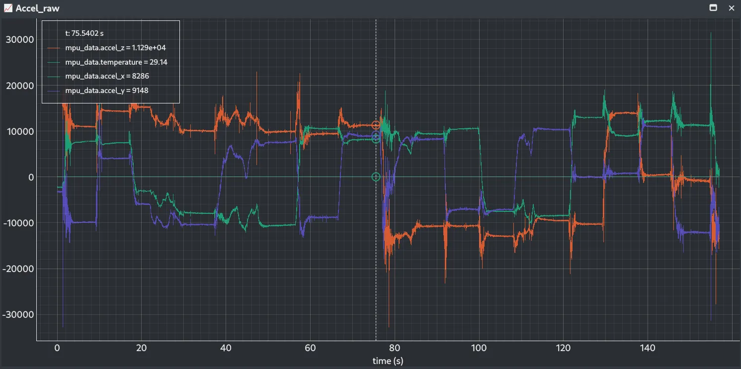The twelve held-out poses as captured. Every one loads all three axes at once, which is where a diagonal model would fail if it were going to.

Pose	Type	N	‖a‖ error, uncalibrated	‖a‖ error, calibrated
1	corner	5447	+0.494%	+0.354%
2	corner	4806	−0.374%	+0.157%
3	corner	5031	+1.886%	+0.491%
4	corner	5221	+1.372%	+0.461%
5	corner	4524	+0.799%	−0.469%
6	corner	6513	+1.061%	−0.683%
7	corner	4835	+0.625%	−0.067%
8	corner	5560	−0.211%	+0.026%
9	edge	5242	+1.110%	−0.594%
10	edge	5428	+1.835%	+0.373%
11	edge	5075	+0.736%	+0.012%
12	edge	5441	+1.085%	−0.186%

“Corner” poses load all three axes at roughly 0.5 g; “edge” poses load two while the third sits near zero.

Calibration improves the worst case from 1.89% to 0.68% and the mean absolute error from 0.97% to 0.32% — about a factor of three.

Note that 0.68% is nearly three times the 0.24% seen at the six calibration positions. That gap is the entire reason for running this test: the six positions flatter the model, because they are the points it was fitted to. Never validate a model only at the points you fitted it with.

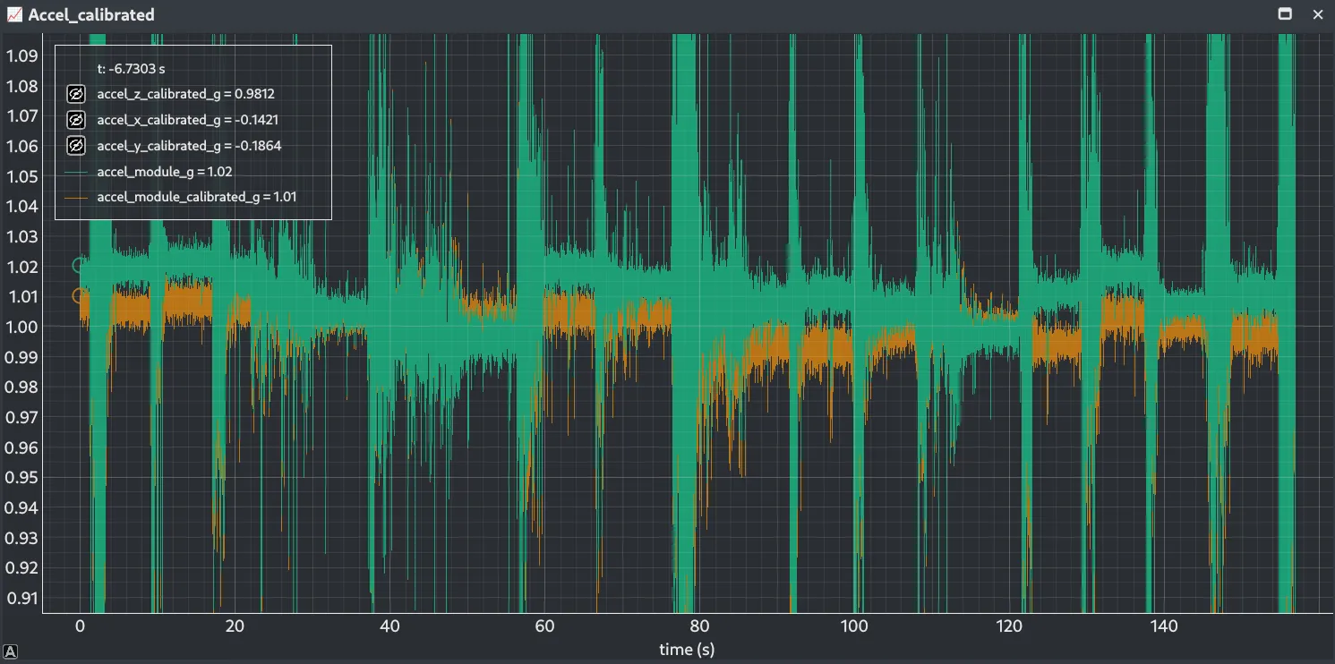The same capture as gravity magnitude. The calibrated trace holds near 1 g across every pose; the uncalibrated one sits high and wanders. The full-height bands are the board being moved between poses.

Where the remaining error comes from

The leftover errors are not random. Every pose with a positive Z component reads high, almost every pose with a negative Z component reads low, and the two poses with Z near zero sit within 0.19% of unity. An error that flips sign with the axis direction is the signature of an offset — a wrong scale factor would push the magnitude the same way at both ends of the axis. That is a useful diagnostic to keep: sign-flipping means bias, same-sign means gain.

Re-fitting the three offsets to these twelve poses, with the scale factors held fixed, confirms it and halves the error:

Fit	RMS error	Worst error
Stored constants from section 5	0.390%	0.683%
Offsets re-fitted, scale fixed	0.185%	0.302%
Offsets and scale both re-fitted	0.154%	0.285%

The Z offset the fit asks for is about 89 LSB above the stored value — the same direction as the drift already measured across a single power cycle, and more of it. Letting the scale factors move too buys almost nothing, and the changes it wants (0.2% to 0.6%) contradict the 0.03% reproducibility measured earlier, so that last row is the fit soaking up offset error, not finding a real sensitivity change.

Corner and edge poses also behave alike — mean error 0.34% against 0.29% — where an unmodelled cross-axis term would have hurt the corner poses most.

So, of the 0.68% worst case: most is offset drift accumulated since the constants were measured, and about 0.3% is what remains once that is removed. The model is not the limiting factor here. The staleness of its offsets is.

What this experiment does not measure

The model used here is diagonal: one bias and one scale factor per axis. The general form is a full 3×3 matrix plus an offset vector, where the off-diagonal terms cover cross-axis sensitivity and axis non-orthogonality.

Those terms are not measured here, and this method cannot measure them. Positioning by nulling drives the off-axis readings to zero by construction, so sensor cross-axis coupling, die-to-package misalignment and residual positioning error all look identical. Telling them apart needs a rotary stage with known reference angles.

What the twelve poses do give is an upper bound. They load all three axes at once, which is where off-diagonal terms would show up, and after re-fitting the offsets the residual is 0.185% RMS and 0.302% at worst. Whatever cross-axis coupling this module has, its effect on the gravity magnitude is no bigger than that — comfortably below the ±2% typical cross-axis sensitivity in the datasheet, though the two are not quite the same quantity. On a low-cost IMU like this one, offset staleness is the problem worth solving first; the matrix form is a subject for a later experiment.

8. Results

Parameter	Before calibration	After calibration
Gravity magnitude error, arbitrary poses	up to 1.89%	up to 0.68%
Gravity magnitude error, six positions	up to 1.37%	up to 0.24%
Axis offset	up to 12.0 mg	corrected; moves up to 2.2 mg per power cycle
Sensitivity error	up to +1.39%	corrected; reproduces to 0.03%

The two magnitude rows differ because the six positions are the points the model was fitted to. The arbitrary poses are the honest figure.

A six-constant model, applied in one line per axis, improved gravity-magnitude accuracy by roughly a factor of three at orientations it had never seen. What error remains is not the model’s fault — it is how far the offsets have drifted since the constants were measured.

9. Implementing the Calibration in Firmware

The arithmetic is one line per axis:

acceleration_g = (raw - bias_lsb) / scale_lsb_per_g;

The reference firmware keeps the six constants in a struct rather than as compile-time constants:

typedef struct {
    float scale[3];   /* LSB/g, X Y Z */
    float bias[3];    /* LSB,   X Y Z */
} MPU6050_Calibration_t;

Both are hardcoded — loaded at startup from guarded defaults in the header, so another module’s numbers can come from the build without touching the driver. Keeping them in RAM rather than in flash costs 24 bytes and buys the same thing section 6 did: the six values can be retuned over SWD, live, without a rebuild.

Hardcoding the bias needs saying out loud, because section 7 measured what it costs. The scale factors are safe — 0.03% across a power cycle, nothing to worry about. The offsets are not: up to 2.2 mg, which by section 7’s re-fit is most of the error that remains after calibration. A stored offset describes the device as it was, not as it is.

For a measurement rig that is the right trade. What you want here is a fixed, known transform — captures taken on different days are comparable because the constants did not move underneath them, and an offset that drifts a couple of milli-g is a fair price for that.

Ship something that has to hold accuracy in the field and the answer flips: re-measure the offsets at startup instead. It is cheap — hold the device still, average a few thousand samples, subtract the expected gravity vector from whichever axis is carrying it. The catch is that the device must be stationary and in a known attitude while it happens. Products that cannot guarantee both ship a user-triggered calibration step instead: the same procedure, with the user supplying the attitude.

So the takeaway is not that constants should be measured rather than assumed. It is that the two have different lifetimes, and treating them the same way should be a decision you made on purpose — harmless in a measurement rig, quietly corrosive in a product.

10. What This Experiment Showed

• Six static positions, roughly ten thousand samples each, are enough to extract bias and scale for all three axes — hand-held, with no jig, no rotary stage and no machined reference surface.
• Nulling the orthogonal axes is a legitimate way to find those positions. The indicator is around a hundred times more sensitive than the error it guards against, which is what makes a hand steady enough.
• Calibration cut the gravity-magnitude error from 1.9% to 0.68% at orientations the model had never seen.
• Checking only the six calibration positions would have reported 0.24% and been misleading. A model reproduces its own fit points by construction; validate somewhere else.
• Scale and bias are not equally trustworthy. Scale reproduced to 0.03% across a power cycle; bias moved by up to 2.2 mg — about ten times the precision the calibration itself achieved. The two constants have different shelf lives, and firmware should treat them as such.
• What error remains is stale offsets, not an inadequate model.

Measurement precision was never the limiting factor. Averaging ten thousand samples pins each calibration point to a couple of LSB — and switching the board off and on again moves it by thirty. That is the number worth designing around.

Every number above came out of firmware that did nothing but read raw counts. The statistics, the model and the validation all ran in EmbedStudio against the live data, which made it cheap to be wrong several times before being right — no rebuild between attempts, and the mistake visible while the board was still in hand. Only then did the constants move into firmware.

References

• InvenSense, MPU-6000 and MPU-6050 Product Specification, Rev. 3.4 (PS-MPU-6000A-00, 2013) — PDF. Source of the nominal 16384 LSB/g at ±2 g that the measured scale factors are compared against in section 5, and of the ±2% typical cross-axis sensitivity discussed in section 7.
• InvenSense, MPU-6000 and MPU-6050 Register Map and Descriptions, Rev. 4.2 (RM-MPU-6000A-00, 2013) — PDF. Source of the register values in section 1, and of the burst-read layout that delivers acceleration and die temperature together.
• Analog Devices, AN-1057: Using an Accelerometer for Inclination Sensing — application note. Derives the same per-axis offset and gain model used in section 5, from the same +1 g and −1 g gravity references.

Next Experiment

Experiment #003: MPU6050 Gyroscope Calibration and Drift Analysis

The accelerometer provides a calibrated gravity vector. The next step is to investigate gyroscope bias and understand how small errors accumulate over time.